Automated Koopman Operator Linearization Library

Project description


AutoKoopman
Overview
AutoKoopman is a high-level system identification tool that automatically optimizes all hyper-parameters to estimate accurate system models with globally linearized representations. Implemented as a python library under shared class interfaces, AutoKoopman uses a collection of Koopman-based algorithms centered on conventional dynamic mode decomposition and deep learning. Koopman theory relies on embedding system states to observables; AutoKoopman provides major types of static observables.
The library supports
- Discrete-Time and Continuous-Time System Identification
- Extended Dynamic Mode Decomposition (EDMD) [Williams et al.]
- Deep Koopman [Li et al.]
- SINDy [Brunton et al.]
- Static Observables
- Random Fourier Features [Bak et al.]
- Polynomial
- Neural Network [Li et al.]
- System Identification with Input and Control
- Koopman with Input and Control (KIC) [Proctor et al.]
- Online (Streaming) System Identification
- Online DMD [Zhang et al.]
- Hyperparameter Optimization
- Random Search
- Grid Search
- Bayesian Optimization
Use Cases
The library is intended for a systems engineer / researcher who wishes to leverage data-driven dynamical systems techniques. The user may have measurements of their system with no prior model.
- Prediction: Predict the evolution of a system over long time horizons
- Control: Synthesize control signals that achieve desired closed-loop behaviors and are optimal with respect to some objective.
- Verification: Prove or falsify the safety requirements of a system.
Installation
The module is published on PyPI. It requires python 3.8 or higher. With pip installed, run
pip install autokoopman
at the repo root. Run
python -c "import autokoopman"
to ensure that the module can be imported.
Examples
A Complete Example
AutoKoopman has a convenience function auto_koopman that can learn dynamical systems from data in one call, given
training data of trajectories (list of arrays),
import matplotlib.pyplot as plt
import numpy as np

# this is the convenience function
from autokoopman import auto_koopman

np.random.seed(20)

# for a complete example, let's create an example dataset using an included benchmark system
import autokoopman.benchmark.fhn as fhn
fhn = fhn.FitzHughNagumo()
training_data = fhn.solve_ivps(
    initial_states=np.random.uniform(low=-2.0, high=2.0, size=(10, 2)),
    tspan=[0.0, 10.0],
    sampling_period=0.1
)

# learn model from data
experiment_results = auto_koopman(
    training_data,          # list of trajectories
    sampling_period=0.1,    # sampling period of trajectory snapshots
    obs_type="rff",         # use Random Fourier Features Observables
    opt="grid",             # grid search to find best hyperparameters
    n_obs=200,              # maximum number of observables to try
    max_opt_iter=200,       # maximum number of optimization iterations
    grid_param_slices=5,   # for grid search, number of slices for each parameter
    n_splits=5,             # k-folds validation for tuning, helps stabilize the scoring
    rank=(1, 200, 40)       # rank range (start, stop, step) DMD hyperparameter
)

# get the model from the experiment results
model = experiment_results['tuned_model']

# simulate using the learned model
iv = [0.5, 0.1]
trajectory = model.solve_ivp(
    initial_state=iv,
    tspan=(0.0, 10.0),
    sampling_period=0.1
)

# simulate the ground truth for comparison
true_trajectory = fhn.solve_ivp(
    initial_state=iv,
    tspan=(0.0, 10.0),
    sampling_period=0.1
)

# plot the results
plt.plot(*trajectory.states.T)
plt.plot(*true_trajectory.states.T)
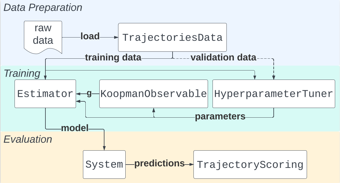
Architecture
The library architecture has a modular design, allowing users to implement custom modules and plug them into the learning pipeline with ease.
Documentation
See the AutoKoopman Documentation.
References
[1] Williams, M. O., Kevrekidis, I. G., & Rowley, C. W. (2015). A data–driven approximation of the koopman operator: Extending dynamic mode decomposition. Journal of Nonlinear Science, 25, 1307-1346.
[2] Li, Y., He, H., Wu, J., Katabi, D., & Torralba, A. (2019). Learning compositional koopman operators for model-based control. arXiv preprint arXiv:1910.08264.
[3] Brunton, S. L., Proctor, J. L., & Kutz, J. N. (2016). Discovering governing equations from data by sparse identification of nonlinear dynamical systems. Proceedings of the national academy of sciences, 113(15), 3932-3937.
[4] Bak, S., Bogomolov, S., Hencey, B., Kochdumper, N., Lew, E., & Potomkin, K. (2022, August). Reachability of Koopman linearized systems using random fourier feature observables and polynomial zonotope refinement. In Computer Aided Verification: 34th International Conference, CAV 2022, Haifa, Israel, August 7–10, 2022, Proceedings, Part I (pp. 490-510). Cham: Springer International Publishing.
[5] Proctor, J. L., Brunton, S. L., & Kutz, J. N. (2018). Generalizing Koopman theory to allow for inputs and control. SIAM Journal on Applied Dynamical Systems, 17(1), 909-930.
[6] Zhang, H., Rowley, C. W., Deem, E. A., & Cattafesta, L. N. (2019). Online dynamic mode decomposition for time-varying systems. SIAM Journal on Applied Dynamical Systems, 18(3), 1586-1609.


Download files
Download the file for your platform. If you're not sure which to choose, learn more about installing packages.
Source Distribution
Built Distribution
Hashes for autokoopman-0.30.4-py3-none-any.whl
| Algorithm | Hash digest | |
|---|---|---|
| SHA256 | eff092b10ec9d430498bbe367f6c7ae821d76b8f3ee5d386c948e4952398982d |
|
| MD5 | 67f8cfcf1f31293ba5f298bd2d0444b8 |
|
| BLAKE2b-256 | c9c411ea66130332e9de3df93d6c56c8bb509d282fe232f8c4436ef2441c952e |


