Machine-learning pipelining and benchmarking suite geared towards the physical sciences.

Project description

Description
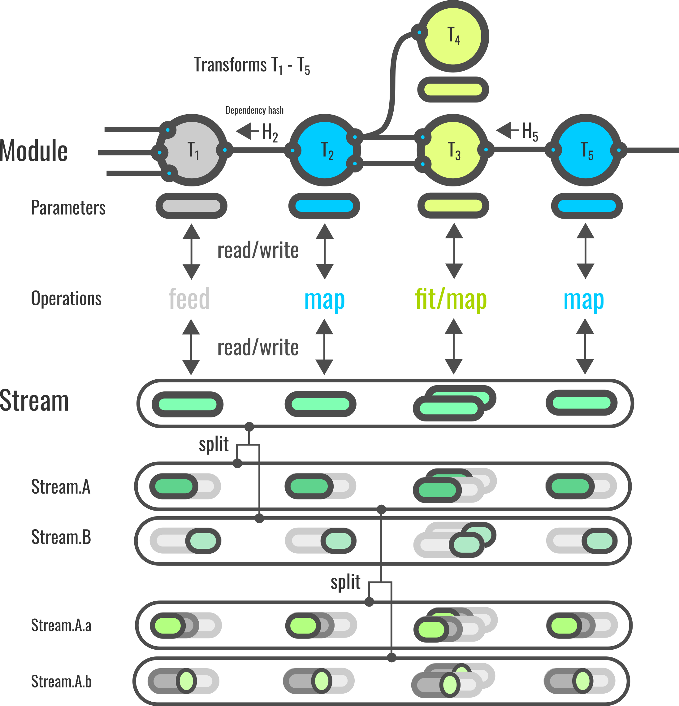
BenchML is a machine-learning (ML) suite for rapid development and deployment of ML models. The library is geared towards physical/chemical datasets and prediction settings. It implements transforms and provides plugins for a variety of atomistic and molecular descriptors, data filtering and feature generation routines, regressors and classifiers, etc. The pipelines can be efficiently optimized using grid-based or Bayesian protocols that minimise recomputation by dependency hashing.
See also our recent manuscript https://arxiv.org/abs/2112.02287, which details an application of BenchML to benchmarking of chemical representations.
Installation
For a minimal installation without plugins, simply
pip install benchml
For a complete installation, create a (new) conda environment from env.yml. E.g.,
git clone https://github.com/capoe/benchml.git
cd benchml
conda env create -n py3benchml -f env.yml
conda activate py3benchml
pip install .
Getting started
In the examples folder, the demo notebook (examples/demo) illustrates how to build simple model pipelines for generic non-molecular datasets. Other examples include ligand activity predictions (examples/ecfp_binding) and a benchmarking workflow (examples/benchmark).
Note that BenchML is being actively developed and still in an alpha state. I.e., the API has not fully equilibrated yet, but we will work on keeping the examples up-to-date as well as making a more detailed documentation available soon.
See the remainder of this page for a description of the key concepts underlying the BenchML framework.
BenchML pipelines
A short guide to ...
Transforms
Transforms are the nodes of the pipeline: They act on the data stream via calls to their .map and/or .fit methods. The results are then stored in their private stream and/or parameter object. An example for the constructor call that creates a new transform instance reads as follows:
trafo = RandomProjector(
    args={
        "cutoff": 0.1,
        "epsilon": 0.01,
        # ...
    },
    inputs={
        "X": "descriptor.x",
        "y": "input.y",
        "M": "predictor._model",
        # ...
    },
)
- The "args" dictionary supplies the parameters of the transformation, such as a cutoff, a convergence threshold, etc. These parameters should not be confused with the output parameters (which could, e.g., include fit coefficients or trained models) stored in the params() object of a transform.
- The "inputs" field contains links to the data stream of ancestral transforms on which the transformation acts. The address of the inputs is specified in the form <transform_tag>.<data_tag>. For example, "descriptor.x" points to the field "x" stored in the stream of the transform with name tag "descriptor". If the tag is prefixed with an underscore "_" (such as in "predictor._model"), then the input is not read from the stream of the respective node, but its params object.
Implementing a new transform class
There are three types of transforms: input, map, and fit+map transforms. Which type we are dealing with is determined by which methods (._feed, ._map, ._fit) a particular transform implements.
Input transforms
Input transforms, such as ExtXyzInput, implement the ._feed method that is called inside .open of a model (= pipeline):
stream = model.open(data)  # < Internally this will call .feed on all
                           #   transforms that implement the ._feed method.
Below we show an example implementation for an input node (here: ExtXyzInput), where .feed is used to release "configs","y" and "meta" into the data stream:
class ExtXyzInput(InputTransform):            # < All transforms derive from <TransformBase>
    allow_stream = {"configs", "y", "meta"}   # < Fields permitted in the stream object
    stream_copy = ("meta",)                   # < See section on class attributes
    stream_samples = ("configs", "y")         # < See section on class attributes

    def _feed(self, data, stream):
        stream.put("configs", data)
        stream.put("y", data.y)
        stream.put("meta", data.meta)
Map transforms
A map transform implements only ._map (but not ._fit). Most descriptors fall within this class of transforms, such as the RandomDescriptor class below:
class RandomDescriptor(Transform):
    default_args = {
      "xmin": -1.0,
      "xmax": +1.0,
      "dim": None
    }
    req_args = ("dim",)           # < Required fields to be specified in the constructor "args"
    req_inputs = ("configs",)     # < Required inputs to be specified in the constructor "inputs"
    allow_stream = {"X"}
    stream_samples = ("X",)
    precompute = True

    def _map(self, inputs, stream):       # < The inputs dictionary comes preloaded with the appropriate data
        shape = (
          len(inputs["configs"]),
          self.args["dim"])
        X = np.random.uniform(
          self.args["xmin"],
          self.args["xmax"],
          size=shape)
        stream.put("X", X) # < The X matrix is stored in the active stream of the transform
Fit transforms
Fit transforms implement ._fit and ._map: The former is called during the training stage within model.fit(stream) The fit stores its parameters in the transform.params() object, but may also access transform.stream(), e.g., to store predicted targets for the training set. The map operation reads model parameters from .params() (e.g. via self.params().get("coeffs")), and releases the mapped output into the stream. See below a wrapper around the Ridge predictor from sklearn:
class Ridge(FitTransform):
    default_args = {"alpha": 1.0}
    req_inputs = ("X", "y")
    allow_params = {"model"}
    allow_stream = {"y"}

    def _fit(self, inputs, stream, params):
        model = sklearn.linear_model.Ridge(**self.args)
        model.fit(X=inputs["X"], y=inputs["y"])
        yp = model.predict(inputs["X"])
        params.put("model", model)
        stream.put("y", yp)

    def _map(self, inputs, stream):
        y = self.params().get("model").predict(inputs["X"])
        stream.put("y", y)
TransformBase class attributes
New transform classes may require us to update their class attributes in order to define default arguments, required inputs, or ensure correct handling of their data streams. The base TransformBase class lists the following class attributes:
class TransformBase(object):
    default_args = {}
    req_args = tuple()
    req_inputs = tuple()
    precompute = False
    allow_stream = {}
    allow_params = {}
    stream_copy = tuple()
    stream_samples = tuple()
    stream_kernel = tuple()
Computationally expensive transforms should typically set "precompute = True", which will add them to the list of transforms mapped during a call to model.precompute(stream). This will precompute the output for a specific data stream, and then only recompute values if the version hash of the stream changes (e.g., due to an args update of an ancestral transform).
For hyperoptimization, as well as benchmarking purposes, the stream attached to a transform needs to know how to split its data into a train and test partition. Consider e.g.,
stream = model.open(data)
model.precompute(stream)
stream_train, stream_test = stream.split(method="random", n_splits=5, train_fraction=0.7)
model.fit(stream_train)
The stream_copy, stream_samples and stream_kernel attributes inform the streamm how to adequately split its member data onto these partitions. For example, for ExtXyzInput, we have the following:
class ExtXyzInput(InputTransform):
    allow_stream = {"configs", "y", "meta"}
    stream_copy = ("meta",)
    stream_samples = ("configs", "y")
This will instruct the split operation to simply copy all the "meta" data to both stream_train and stream_test, whereas the "configs" and "y" data listed in "stream_samples" will be sliced (such as in configs_train = configs[trainset], configs_test = configs[testset]).
Finally, for a precomputed kernel object, this slicing operation differs qualitatively from slicing of, say, a design matrix, as this affects the two axes of the matrix in different way e.g., K_train = K[trainset][:,trainset], where K_test = K[testset][:,trainset]. This is why the kernel matrix computed, e.g.,by the KernelDot transform is listed in a dedicated stream_kernel attribute:
class KernelDot(FitTransform):
    default_args = {"power": 1}
    req_inputs = ("X",)
    allow_params = {"X"}
    allow_stream = {"K"}
    stream_kernel = ("K",)
    precompute = True
How to add a plugin
New transforms can be defined either externally or internally. In the latter case, add a source file with the implementation to the benchml/plugins folder, and ,subsequently, import that file in benchml/plugins/init.py. You can check that your transforms were successfully added using bin/bmark.py:
./bin/bmark.py --list_transforms
Modules
A module (also referred to as a pipeline or model) comprises a set of interdependent transforms, with at least one input transform. The module applies the transforms sequentially to the data input during the fitting and mapping stages, managing both data streams and parameters.
The code example below creates a new pipeline instance that combines a topological fingerprint with a dot-product kernel and kernel ridge regression:
model = Module(
    tag="morgan_krr",
    transforms=[
        ExtXyzInput(tag="input"),                 # < By assigning the tag "input", the stream
        TopologicalFP(                            #   from ExtXyzInput can be accessed via "input.<field>"
            tag="descriptor",                     #   instead of "ExtXyzInput.<field>".
            inputs={"configs": "input.configs"}),
        KernelDot(
            tag="kernel",
            inputs={"X": "descriptor.X"}),
        KernelRidge(
            args={"alpha": 1e-5, "power": 2},
            inputs={"K": "kernel.K", "y": "input.y"})
    ],
    hyper=BayesianHyper(
        Hyper({
            "KernelRidge.alpha": [-3, 3 ],
            "KernelRidge.power": [ 1., 3. ]}),
        convert={
            "KernelRidge.alpha": lambda a: 10**a}),
    broadcast={ "meta": "input.meta" },           # < Data objects referenced here are broadcast to
    outputs={ "y": "KernelRidge.y" },             #   all transforms, and can be accessed via the
)                                                 #   inputs argument in their .\_map and .\_fit methods.
Note that except for "transforms", all arguments in this constructor are optional. Still, most pipelines will typically define some "outputs", that are returned as a dictionary after calls to model.map(stream). Hyperparameter optimization is added via "hyper". In the example above, a grid search over the kernel ridge parameters "alpha" and "power" will be performed within model.hyperfit(stream, ...). Calls to model.fit(stream) on the other hand would only consider the transform args specified in the "transforms" section of the constructor.
Using the module
In the simpler .fit case, where a model is to be parametrized on some predefined training data, and then applied to a prospective screen, the workflow would simply be:
stream_train = model.open(data_train)
model.fit(stream_train)
stream_screen = model.open(data_screen)
output = model.map(stream_screen)
print("Predicted targets =", output["y"])
If hyperparameter optimization is desired, the type of nested splits as well as an evaluation metric need to be specified. It is then usually a good idea to call model.precompute before model.hyperfit in order to cache data (such as, e.g., a design matrix) that do not change during the hyperparameter sweep:
stream_train = model.open(data_train)
model.precompute(stream_train)
model.hyperfit(
    stream=stream_train,
    split_args={"method": "random", "n_splits": 5, "train_fraction": 0.75},
    accu_args={"metric": "mse"},  # < These arguments are handed over to an "accumulator"
    target="y",                   #   that evaluates the desired metric between the target "y"
    target_ref="input.y")         #   (read from the model output) and reference "input.y"
                                  #   (read from the stream of the "input" transform).
Accessing data within a stream or module
The methods model.open(data) as well as stream.split(...) return handles on a data stream. You can manually access the data stored in the stream via
X = stream.resolve("descriptor.X")
y_true = stream.resolve("descriptor.y")
You can also obtain data and model parameters from an active stream and params objects through the model:
y_pred = model.get("KernelRidge.y")
predictor = model.get("KernelRidge._model")
The underscore "_" indicates that the "model" data is to be read from the .params() of the KernelRidge transforminstead of the .stream().
Macros
Certain transform sequences may reappear in various models in the same way. It can then be convenient to implement a macro that behaves like a single transform class when supplied to the constructor of a new module. Below we show how to combine a topological fingerprint with a dot-product kernel within a single macro:
class TopologicalKernel(Macro):
    req_inputs = ("descriptor.configs",)
    transforms = [
        {
            "class": TopologicalFP,
            "tag": "descriptor",
            "args": {"length": 1024, "radius": 3},
            "inputs": {"configs": "?"},
        },
        {
            "class": KernelDot,
            "tag": "kernel",
            "args": {},
            "inputs": {"X": "descriptor.X"}
        }
    ]
This macro can then be used by a module that, e.g., sums two kernels with different hyperparameters into a single kernel using the "Add" transform:
Module(
    transforms=[
        ExtXyzInput(tag="input"),
        TopologicalKernel(
            tag="A",
            args={"descriptor.fp_length": 1024, "descriptor.fp_radius": 2},
            inputs={"descriptor.configs": "input.configs"},
        ),
        TopologicalKernel(
            tag="B",
            args={"descriptor.fp_length": 2048, "descriptor.fp_radius": 4},
            inputs={"descriptor.configs": "input.configs"}
        ),
        Add(
            args={"coeffs": [ 0.5, 0.5 ]},
            inputs={"X": ["A/kernel.K", "B/kernel.K"]}
        ),
        KernelRidge(
            args={"alpha": 0.1, "power": 2},
            inputs={"K": "Add.y", "y": "input.y"}
        ),
    ]
)
Note that streams within the macros are located within their own namespace. Hence, the kernel from transform "A" is referenced outside the macro via "A/kernel.K" instead of just "kernel.K".
Hyper-optimization
The library currently allows grid-based and Bayesian hyperparameter optimization. These are added to the model definition via the "hyper" argument of the constructor. A grid-based example reads as follows:
model = Module(
    transforms=[
        # ...
        KernelRidge(...)
        # ...
    ],
    hyper=GridHyper(
        Hyper({ "KernelRidge.alpha": np.logspace(-3,+3, 5), }),
        Hyper({ "KernelRidge.power": [ 1., 2., 3. ] })),
),
As there are two independent objects within the GridHyper constructor, a complete combinatorial sweep will be performed, testing all combinations of "KernelRidge.alpha" and "KernelRidge.power" (here: 5x3 = 15). Hyperparameters contained within the same Hyper object, by contrast, are swept over in a linear fashion:
model = Module(
    transforms=[
        # ...
        KernelRidge(...)
        # ...
    ],
    hyper=GridHyper(
        Hyper({
            "KernelRidge.alpha": np.logspace(-3,+3, 3), # < Only three combinations considered:
            "KernelRidge.power": [ 1., 2., 3. ]         #   (alpha, power) = (-3,1), (0,2), (3,3)
        }))
)
As the number of hyperparameters increases, the grid-based sweep becomes increasingly expensive. Bayesian optimization can then be a more efficient choice:
model = Module(
    transforms=[
        # ...
        KernelRidge(...)
        # ...
    ],
    hyper=BayesianHyper(
        Hyper({
            "KernelRidge.alpha": [ -3, 3 ],
            "KernelRidge.power": [ 1.0, 3.0 ] }),
        convert={"KernelRidge.alpha": lambda a: 10**a}),
),
Here we specified the lower and upper limit for each hyperparameter. The "convert" dictionary contains instructions that are applied to a hyperparameter before it is supplied to the module: For example, "KernelRidge.alpha" is exponentiated with base 10, such that the Bayesian optimization (which is hence applied to the log of the regularization alpha) experiences a smoother landscape. A similar conversion is necessary when integral or boolean parameters are to be optimized:
# ...
hyper=BayesianHyper(
    Hyper({
        "trafo.some_boolean": [ 0.0, 1.0 ],
        "trafo.some_integer": [ 128, 512] }),
    convert={
        "trafo.some_boolean": lambda b: bool(np.round(b)),
        "trafo.some_integer": lambda f: int(f)
    })
# ...
Development
Tests
The tests are split onto unit and end-to-end (e2e) tests:
python3 -m pytest tests/unit_tests
python3 tests/e2e_tests/test_all.py
Adding --create to the second command will generate reference results.
To run a juypter notebook as a test, do
pip install nbmake
python3 -m pytest --nbmake "examples/"
Release history Release notifications | RSS feed


Download files
Download the file for your platform. If you're not sure which to choose, learn more about installing packages.
Source Distribution
Built Distribution
Hashes for BenchML-0.3.4-py2.py3-none-any.whl
| Algorithm | Hash digest | |
|---|---|---|
| SHA256 | 1cdc7e3b579164646b8fe9dcccd727ef3af7672ca091a8bf0de98e9bac1bfd29 |
|
| MD5 | 9e641772e12a54ca7745481323449d69 |
|
| BLAKE2b-256 | 59e782ded728e470a6e63e884ba9565e8c9a5a830f3665048f61736d0a4ae748 |


