DAQData

Usage

Read and plot slow and fast data binary files from centrifuge experiments conducted at Center of Geotechnical Modeling at University of California Davis

Features

• Reads slow and fast data binary files.
• List downs all the sensors,channels,configuration list, sampling rate...
• Extract all data or a subset of a data within a time frame as a pandas DataFrame object
• Plot data directly from the binary file.
• supports reading and plotting large data files.

Installation

This package is availably via pypi:

pip install DAQData

Read meta data from the binary file

import DAQData as DQ;

# Centrifuge CGM (UC Davis) data file. Can be slow as well as fast data 
Data_File = "./Binary_Data_Files/07122019@121326@154548@64.4rpm.bin";

# By default the, 'Extract_Data' parameter is set to be True. If the files are
# very large and only meta data needs to be checked, the data extraction can be
# stooped by setting 'Extract_Data' parameter false. This would increase the
# execution speed but will not read any data 
Data_DAQ = DQ.DAQ(Data_File,Extract_Data=True);

# To print all the meta data 
print(Data_DAQ)


# Extracting meta data
FileName                      = Data_DAQ.FileName; # gets the filename
Sampling_Rate                 = Data_DAQ.Sampling_Rate; # gets Sampling_Rate
Number_of_Channels            = Data_DAQ.Number_of_Channels; # gets number of channels
Number_of_Hardware_Channels   = Data_DAQ.Number_of_Hardware_Channels; # gets number of hardware channels
Number_of_Sensors             = Data_DAQ.Number_of_Sensors # gets number of Xdcr_Serial Numbers (also referred as sensors)
Channel_List                  = Data_DAQ.Channel_List; # gets the channel list
Hardware_Channel_List         = Data_DAQ.Hardware_Channel_List; # get the hardware channel list
Sensor_List                   = Data_DAQ.Sensor_List; # gets the sensor list 
Number_of_Samples             = Data_DAQ.Number_of_Samples; # gets the total number of samples per sensor 
Data_Length                   = Data_DAQ.Data_Length; # gets the total data length in the binary file. Number_of_Samples*Number_of_sensors
Channel_Dictionary            = Data_DAQ.Channel_Dictionary; # returns a dictionary of channel name to the column number in the Channel List  
ExcelConfig                   = Data_DAQ.ExcelConfig; # return excel configuration file as a csv string 

Extract data on demand

import DAQData as DQ;

Data_File = "./Binary_Data_Files/07122019@121326@154548@64.4rpm.bin";
Data_DAQ  = DQ.DAQ(Data_File,Extract_Data=True);


# If the 'Extract_Data' parameter is True, the whole data is already read and extracted and can be easily retrieved as
Sensor_Data         = Data_DAQ.Sensor_Data;	# 2-D pandas DataFrame with column names (headers) as Channel Names 
print(Sensor_Data.head(2)); # shows first 2 rows of the data set
# print(Sensor_Data.shape); # gets the size of the dataset (rows,columns)
# print(Sensor_Data['ICP1-0']) # will retrieve the data for channel no  'ICP1-0'
# print(Sensor_Data.columns) # will show all the header names in the data. It is the same as the Channel List. 

# The column names can be renamed to sensor names or any other meaningful names as shown below
Sensor_Data.columns = ["TIME (s)","EAST (g)","WEST (g)","P1_ACC_H2 (g)","P2_ACC_H2 (g)","P1_G1 (lbf)","P1_G2 (lbf)","P1_G3 (lbf)","P1_G4 (lbf)","P1_G5 (lbf)","P1_G6 (lbf)","P1_G7 (lbf)","P1_G8 (lbf)","P2_ACC-V1 (g)","P2_ACC_H1 (g)","4th RING (g)","SOUTH (g)","P1_ACC_H1 (g)","P1_ACC_V1 (g)","NORTH (g)","P2_G1 (lbf)","P2_G2 (lbf)","P2_G3 (lbf)","P2_G4 (lbf)","P2_G5 (lbf)","P2_G6 (lbf)","P2_G7 (lbf)","P2_G8 (lbf)","P1_G9 (lbf)","P2_G9 (lbf)","dummy3","Dummy_2","PPT_5 (kPa)","PPT_3 (kPa)","PPT_9 (kPa)","PPT_1 (kPa)","PPT_8 (kPa)","PPT_6 (kPa)","PPT_2 (kPa)","PPT_7 (kPa)","PPT_5442","PPT_4 (kPa)","PPT_10 (kPa)","PPT_10_Proxy (kPa)","Dummy-127926","ACC_6 (g)","ACC_1 (g)","ACC_3 (g)","ACC_5 (g)","ACC_2 (g)","ACC_7 (g)","ACC_4 (g)","dummy21320","dummy-108849","PT 9F008","P2_LP (mm)","P2_MEM (g)","SM2 (mm)","P1_MEM (g)","P1_LP (mm)","SM1 (mm)","PPT_22 (kPa)","PPT_14 (kPa)","PPT_16 (kPa)","PPT_15 (kPa)","PPT_21 (kPa)","MS5407_115","PPT_18 (kPa)","PPT_20 (kPa)","PPT_19 (kPa)","PPT_12 (kPa)","PPT_1 (kPa)","PPT_11 (kPa)","PPT_17 (kPa)","CPT (lbf)","EXT (lbf)","PLT (lbf)","ACT (mm)"]; # here as an example the channel names 'ICP1-0' is renamed to 'EAST (g)'
print(Sensor_Data.head(2)); # shows first 2 columns of the data with new column names
# print(Sensor_Data['EAST (g)']) # will retrieve the data corresponding to column name  'EAST (g)'. Will give the same result (print(Sensor_Data['ICP1-0'])) has the headers or column names not renames 

# If the 'Extract_Data' parameter was initially set to False, the data can be extracted on demand by defining the start and end time
# ..... Time_Data, Sesnor_Data = Data_DAQ.Extract(Start_Time=0, End_Time=10)
# To extract the whole data, set the start time to be 0 and end time to be Number_of_Samples/Sampling_Rate

Data_DAQ  = DQ.DAQ(Data_File,Extract_Data=False);
Sensor_Data = Data_DAQ.Extract(Start_Time=0,End_Time=Number_of_Samples/Sampling_Rate);

# print(Sensor_Data.shape) # would return the same length of data as above 

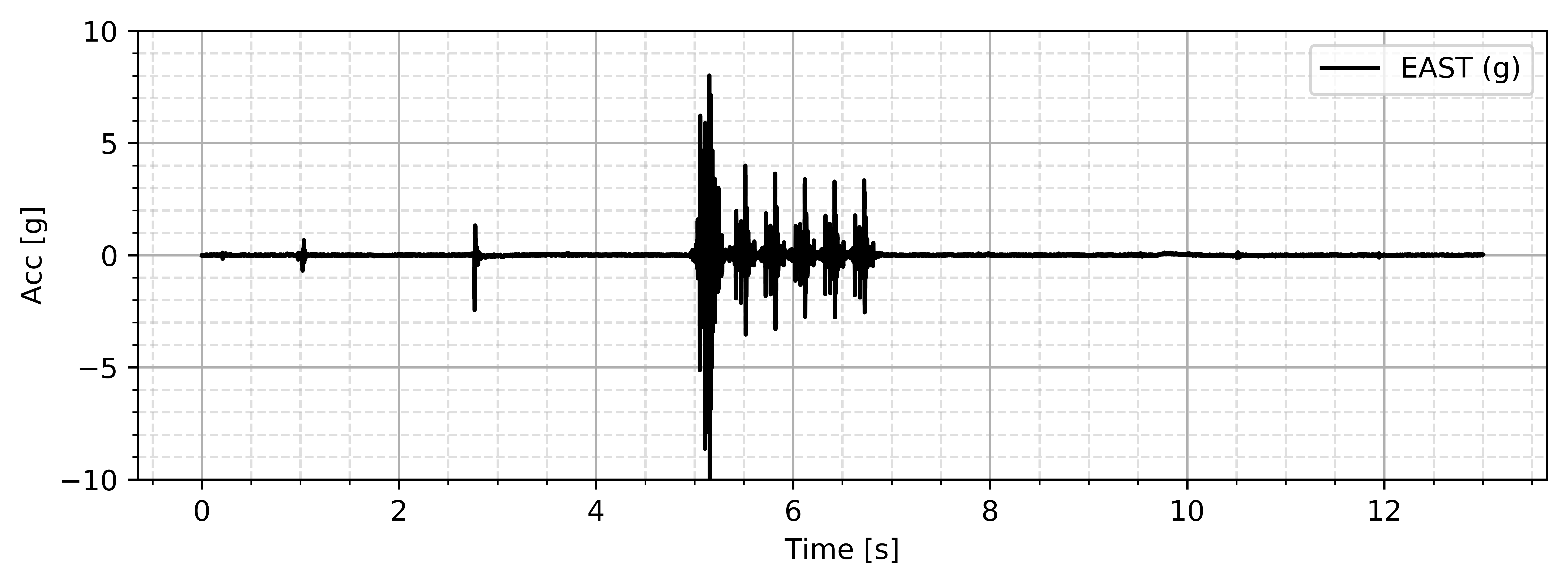
Plot data

import DAQData as DQ;

Data_File = "./Binary_Data_Files/07122019@121326@154548@64.4rpm.bin";
Data_DAQ  = DQ.DAQ(Data_File,Extract_Data=True);

Sensor_Data = Data_DAQ.Sensor_Data;

# get the time data 
Time_Data   = Sensor_Data['TIME']; 
# if the headers were changed as in the previous above examples 
# it can be extracted as Time_Data   = Sensor_Data['TIME (s)']; 

# get the sensor data of interest
# extract the data from the Sensor_Data DataFrame
Input_Acceleration    = Sensor_Data['ICP1-0'];
# if the headers were changed as in the previous above examples 
# it can be extracted as Time_Data   = Sensor_Data['EAST (g)']; 

# extract the sensor name
Sensor_Name   = Data_DAQ.Sensor_List[Data_DAQ.get_Channel_Index(Channel_Name='ICP1-0')];

import matplotlib.pyplot as plt;

plt.figure(figsize=(8,3));
plt.plot(Time_Data,Input_Acceleration,'k',label=Sensor_Name);
plt.legend(loc='best')
plt.grid(axis='both', which='major', ls='-')
plt.grid(axis='both', which='minor', ls='--', alpha=0.4)
plt.minorticks_on()
plt.xlabel('Time [s]')
plt.ylabel('Acc [g]')
plt.ylim([-10,10])
plt.tight_layout();
plt.show();

Send your comments, bugs, issues and features to add to Sumeet Kumar Sinha at sumeet.kumar507@gmail.com. Please feel free to create issues on https://github.com/SumeetSinha/DAQData/issues