Package to handle davis data files

Project description
ddr_davis_data
Pakcage uses lvreader(1.2.0) to read and write .set file of Davis. lvreader is not installed with the package and hence it has to be installed separately. lvreader is not available on pypi (as of Sept 2022).
Download and install lvreader
Download .zip file of lvreader(1.2.0) from here
Extract the .zip file. lvreader has good manual to understand its usage. For independent use of lvreader, user can follow the manual. We will install the lvreader in our sytem from the .whl (wheel) files. Inside there are multiple .whl files. According to the python version, the resective file needs to be installed. for Python 3.9.0 install lvreader-1.2.0-cp39-cp39-win_amd64.whl. For Python 3.10 install lvreader-1.2.0-cp310-cp310-win_amd64.whl.
Above instructions assumes Windows as OS. For Linux the .whl file name changes which is easily distinguishable in the list of files.
Then open Anaconda powershell or cmd.exe. navigate to the extracted folder and perform the installation using pip.
pip install lvreader-1.2.0-cp310-cp310-win_amd64.whl
Select the file name according to the Python version or-else the error will come.
We have installed lvreader and all its required dependecies in the system. Now we will install ddr_davis_data
Install ddr_davis_data
Install ddr_davis_data using pip.
pip install ddr_davis_data
Instantiation
import ddr_davis_data
import matplotlib.pyplot as plt
import numpy as np
import os

print(ddr_davis_data.version)
0.1.19
We need the filepath to Davis set. Here, we will take one average velocity set file. In Davis the files are arranges in chronological manner. The base or the first set (folder containing files) is of recorded images. Then folder inside the base set can be anything depending upon the processing performed. If background image is subtracted then, the next folder would contain subtracted images. Then next folder inside that folder would be instantaneous and then average velocity folder. The hierarchy of the folder depends upon the processing sequence performed. For the case shown here, the hierarchy is as follows.
recorded images
│   .im7 files - all images (from 0 to 100 or 1000)
│   ...
|   background subtracted images.set
└───background subtracted images
    │   .im7 files
    │   ...
    |   instantaneous velocity fields.set
    └───instantaneous velocity fields
        │   .vc7 files containing Vx, Vy or Vz (depending upon type of PIV)
        │   ...
        |   average velocity field.set
        └───average velocity field
            │   .vc7 files containing average of Vx, Vy or Vz (depending upon type of PIV)
            │   ... another files depending upon the processing
In this case, we will take instantaneous set file. The set file is located in the parent directory of the folder as shown above. For the filepath, we can either give the path to .set file or folder path.
filepath1 = r'D:\recorded images\background subtracted images\instantaneous velocity fields'
s1 = ddr_davis_data.velocity_set(filepath = filepath1, load=True, rec_path=None, load_rec=False)
s1 is the velocity set object. If the set folder is in hierarchy of the recorded image, then load_rec=True will load the recording set as well. Loading recording set helps in accessing recoded or raw images. To make the instantiation of velocity_set faster with recording set, it is better to give recoding set folder-path directly to rec_path attribute above.
Accessing data
Every set file has many of attributes such as scales, offsets, limits, U0, V0, camera exposure time, Laser power, recording time, recording rate etc..
s1.attributes
This will give the dictionary-like data of all the attributes attached with the s1 set file. There are default and intuitive functions to get certain important attributes as follows.
len(s1)
100
This gives the number of images in the velocity set.
s1.recording_rate
10.0
gives the recording rate of the s1 set file. similary the time delta in between the frames can be accesssed by,
s1.dt
49.0
Depending upon the way Davis packs the data, sometimes the attribute name changes and then the above functions might not work. At that time it is better to access data using
s1.attributes
Velocity data
Velocity data can be accessed by giving comonent name. Method returns the numpy_masked_array like data.
s1.u(n=0)
masked_array(
  data=[[--, --, --, ..., --, --, --],
        [--, --, --, ..., --, --, --],
        [--, --, --, ..., --, --, --],
        ...,
        [--, --, --, ..., --, --, --],
        [--, --, --, ..., --, --, --],
        [--, --, --, ..., --, --, --]],
  mask=[[ True,  True,  True, ...,  True,  True,  True],
        [ True,  True,  True, ...,  True,  True,  True],
        [ True,  True,  True, ...,  True,  True,  True],
        ...,
        [ True,  True,  True, ...,  True,  True,  True],
        [ True,  True,  True, ...,  True,  True,  True],
        [ True,  True,  True, ...,  True,  True,  True]],
  fill_value=0.0)
This is the $V_x$ velocity with masks. Mask crops the useful data from the overall image. During velocity calculation in Davis if Mask is enabled (geometric mask) then the output velocities will have mask accordingly. Mostly PIV frames are not 100% used for velocity measurements. Meaning if jet is flowing from center of the image then the corners of the image is rendered useless for velocity measurement. Masks helps in neglecting those areas. It only considers the area of interest.
Similarly $V_y$ can be accessed as follows.
s1.v(n=21)
masked_array(
  data=[[--, --, --, ..., --, --, --],
        [--, --, --, ..., --, --, --],
        [--, --, --, ..., --, --, --],
        ...,
        [--, --, --, ..., --, --, --],
        [--, --, --, ..., --, --, --],
        [--, --, --, ..., --, --, --]],
  mask=[[ True,  True,  True, ...,  True,  True,  True],
        [ True,  True,  True, ...,  True,  True,  True],
        [ True,  True,  True, ...,  True,  True,  True],
        ...,
        [ True,  True,  True, ...,  True,  True,  True],
        [ True,  True,  True, ...,  True,  True,  True],
        [ True,  True,  True, ...,  True,  True,  True]],
  fill_value=0.0)
n is the image number for which velocity is enquired. If there are 100 images then n ranges from 0 to 99. As s1 is instantaneous set file, it contains many .vc7 files. But for average set file, there will be only one .vc7 file which will have average of velocity components, then n should be 0 (which is its default value).
s1.vector_coords(n=0)
x= [[-1.         -0.99659864 -0.99319728 ... -0.00680272 -0.00340136
   0.        ]
 [-1.         -0.99659864 -0.99319728 ... -0.00680272 -0.00340136
   0.        ]
 [-1.         -0.99659864 -0.99319728 ... -0.00680272 -0.00340136
   0.        ]
 ...
 [-1.         -0.99659864 -0.99319728 ... -0.00680272 -0.00340136
   0.        ]
 [-1.         -0.99659864 -0.99319728 ... -0.00680272 -0.00340136
   0.        ]
 [-1.         -0.99659864 -0.99319728 ... -0.00680272 -0.00340136
   0.        ]]
y= [[ 0.          0.          0.         ...  0.          0.
   0.        ]
 [-0.00452489 -0.00452489 -0.00452489 ... -0.00452489 -0.00452489
  -0.00452489]
 [-0.00904977 -0.00904977 -0.00904977 ... -0.00904977 -0.00904977
  -0.00904977]
 ...
 [-0.99095023 -0.99095023 -0.99095023 ... -0.99095023 -0.99095023
  -0.99095023]
 [-0.99547511 -0.99547511 -0.99547511 ... -0.99547511 -0.99547511
  -0.99547511]
 [-1.         -1.         -1.         ... -1.         -1.
  -1.        ]]
Returns tuples of numpy-array like data. The data is mesh-grid of $X$ and $Y$ coordinates of velocity vectors.
Plotting
Contour, Streamline, Quiver etc. plots can be made from the meshgrid coordinate data and velocity vector data which we accessed above. There are special methods which is described below to output the data for plots and also there are plotting functions in the library to directly plot the data.
s1.plot(n=10)
Above code directly access the lvreader.frame.VectorFrame.plot() function. There are separate functions in the module to plot various informations.
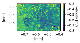
Plot filled contour
ddr_davis_data.plot_contourf(*args,**kwargs) is used to plot filled contour. There are 2 ways to use the function.
1) Giving velocity_set as input
fig = plt.figure(figsize=(3,1.5))
ax = fig.add_subplot(111)

ddr_davis_data.plot_contourf(ax=ax, vel_set=s1, n=10, z='velocity_magnitude', font_size=7,
                            ctitle='|V|',clabel='[m/s]',labelpad=10)
plt.show()
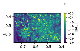
n is the image/frame number. z determines which scalar to plot. There are many options to that depending upon the Davis output file. Currently 'u,v,velocity_magnitude, omega_z, Wz, TKE' options are available. There is a workaround this method of plotting which we will see shortly. Other attributes can be understood from its name or from plot outcome.
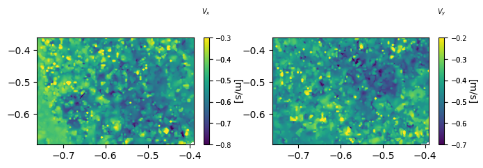
Multiple axes
ax is the axes on which to plot the contour. If there are multiple subplots then this attribute is very helpful. Below code plots the $V_x$ and $V_y$ in two different subplots.
fig = plt.figure(figsize=(8,2))

ax1 = fig.add_subplot(121)
ddr_davis_data.plot_contourf(ax=ax1, vel_set=s1, n=7, z='u', font_size=10,
                             ctitle='$V_x$',clabel='[m/s]',labelpad=10)

ax2 = fig.add_subplot(122)
ddr_davis_data.plot_contourf(ax=ax2, vel_set=s1, n=7, z='v', font_size=10,
                             ctitle='$V_y$',clabel='[m/s]',labelpad=10)

plt.show()
2) Giving data as input
This method of plotting gives better control over the data to be plotted. In the previous example, we gave velocity_set as input. The plotting function makes the data inside using z value. If we make the data outside the function and give the data to plotting function then it will do the same thing, but we could do multiple mathematical manipulation of data before plotting.
data should be dictionary like object.
d1 = s1.make_data(n=10)
Gives the dict output with 'x','y','u' and 'v' keys with numpy_masked array like values. To make the data ready for plotting d1['z'] should be set to the scalar which we want to plot.
fig = plt.figure(figsize=(8,2))
d1 = s1.make_data(n=10)

ax1 = fig.add_subplot(121)
d1['z'] = d1['u']
ddr_davis_data.plot_contourf(ax=ax1,data=d1,font_size=7,ctitle='$V_x$ [m/s]')

ax2 = fig.add_subplot(122)
d1['z'] = d1['v']
ddr_davis_data.plot_contourf(ax=ax2,data=d1,font_size=7,ctitle='$V_y$ [m/s]')

plt.show()
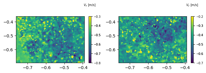
This will plot the same figure as plotted previously using velocity_set. Now here we could do mathematical manipulation of data before storing it to d1['z']. If both vel_set and data are defined then data is given the priority above vel_set.
Common colorbar and use of vmax and vmin
vmax and vmin comes handy when we want to plot common colorbar for multiple subfigures. below code shows the example for the same.
vmin= -1
vmax= 0
colormap='hot'

fig = plt.figure(figsize=(5,1.5))

d1 = s1.make_data(n=10)

ax1 = fig.add_subplot(121)
d1['z'] = d1['u']
ddr_davis_data.plot_contourf(ax=ax1,data=d1,
                             vmax=vmax,vmin=vmin,add_colorbar=False,colormap=colormap)


ax2 = fig.add_subplot(122)
d1['z'] = d1['v']
ddr_davis_data.plot_contourf(ax=ax2,data=d1,
                             vmax=vmax,vmin=vmin,add_colorbar=False,colormap=colormap)

plt.tight_layout()
#adding colorbar to the right
plt.subplots_adjust(right=0.85)
ax = fig.add_axes([0.92,0.05,0.015,0.85])
ddr_davis_data.plot_colorbar(vmin=vmin,vmax=vmax,cax=ax,font_size=7,colormap=colormap,roundto=2,ctitle='$Common$ [m/s]')

plt.show()
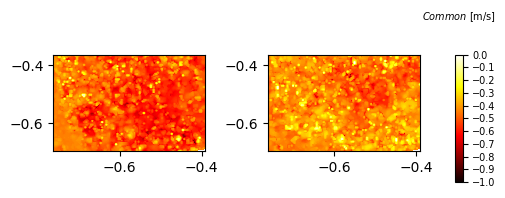
In the above plots we have changed the type of colormap to hot.
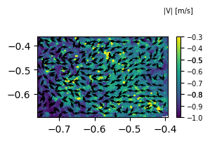
Plot quiver (vectors)
The method to plot the quiver is almost same as above. It shares the same code architechture. There is difference in fracx and fracy attributes, which controlls the amount of vectors displayed in $X$ and $Y$ axes respectively. The higher the number, less the amount of vectors displayed.
Vectors makes more sense when displayed over the contour plot. Hence below figure will plot vectors over the contour plot.
fig = plt.figure(figsize=(3,1.5))
ax1 = fig.add_subplot(111)

d1 = s1.make_data(n=10)
#calculating velocity_magnitude
d1['z'] = (d1['u']**2 + d1['v']**2)**0.5

#plotting contour of velocity magnitude
ddr_davis_data.plot_contourf(ax=ax1,data=d1,font_size=7,ctitle='|V| [m/s]')
#plotting vectors, here the width and scale are adjusted for better vision
ddr_davis_data.plot_quiver(ax=ax1,data=d1,fracx=5,fracy=5,scale=20,width=0.007,color='#000000ff',normalize=True)
plt.show()
normalize = True attribute will normalize the velocity values. This helps when the velocity magnitudes changes very much within the plot.
Plot streamlines
When data from s1.make_data() is supplied to matplotlib.pyplot.streamplot() then error of strictly increasing array pops up. Hence turnaround was to use 1D linear array. There is special function within the velocity_set object which gives the data to plot for streamlines.
fig = plt.figure(figsize=(3,1.5))

ax1 = fig.add_subplot(111)
d1 = s1.make_data(n=10)
d1['z'] = (d1['u']**2 + d1['v']**2)**0.5

ddr_davis_data.plot_contourf(ax=ax1,data=d1,font_size=7,ctitle='|V| [m/s]')
d1 = s1.make_streamline_data(n=10)
ddr_davis_data.plot_streamlines(ax=ax1,data=d1,density=(5,5),linewidth=1,color='white',arrowsize=0.01)
plt.show()
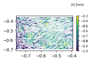
here arrowsize is 0.01 for better visualization. But for some cases, default arrowsize gives good results.
get $\omega_z$
There is a function to calculate $\omega_z$ from the data. The function accepts the data in dict like object form.
d1 = s1.make_data(n=0)
d1 = get_omega_z(data=d1)
d1['z'] contains the calculated $\omega_z$ from the given data. You can further use this dict like data in plotting or any analysis.
Similarly there is function get_mod_V which accepts the same dict like data, and calculates the velocity magnitude. As this calculation is one line and you can do it easily, the usage of function is not specifically described here.
Accessing recording images
Recording images can be accessed if load_rec=True in instantiation of velocity_set object. Also there should be recording .set files in the parent directory (at any level) of the velocity set file.
s1 = ddr_davis_data.velocity_set(filepath = filepath1, load=True, rec_path=None, load_rec=True)
plotting the image
The structure to plot image is similar to contour plot.
- make the data
d1 = s1.make_image_data(n=10) - plot the data
ddr_davis_data.plot_image(data=d1)
fig = plt.figure(figsize=(3,1.5))
ax1 = fig.add_subplot(111)

d1 = s1.make_image_data(n=10,frame=0)
ddr_davis_data.plot_image(ax=ax1,data=d1,vmin=0,vmax=60)
plt.show()
Rotate bases
Davis considers the $V_x$ in horizontal direction and $V_y$ in vertical direction. But for some cases, the physical bases (coordinate system) can be different. Say, $45^{\circ}$. Then we need to project our vectors in that perticular bases. rotate_bases() function does the work for us. Rotation angle must be in degrees.
vmin= -1
vmax= 1
colormap='cool'

fig = plt.figure(figsize=(5,1.5))

ax1 = fig.add_subplot(121)
d1 = s1.make_data(n=25)
d1['z'] = d1['u']
ddr_davis_data.plot_contourf(ax=ax1,data=d1,
                             vmax=vmax,vmin=vmin,add_colorbar=False,colormap=colormap)
ax1.set_title('original bases')

ax2 = fig.add_subplot(122)

# this function rotates the bases
d1 = ddr_davis_data.rotate_bases(d1,angle=45)

ddr_davis_data.plot_contourf(ax=ax2,data=d1,
                             vmax=vmax,vmin=vmin,add_colorbar=False,colormap=colormap)
ax2.set_title('rotated bases')

plt.tight_layout()
plt.subplots_adjust(right=0.85)
ax = fig.add_axes([0.92,0.05,0.015,0.85])
ddr_davis_data.plot_colorbar(vmin=vmin,vmax=vmax,cax=ax,font_size=7,
                             colormap=colormap,roundto=2,ctitle='$V_x$ [m/s]',cticks=5)

plt.show()
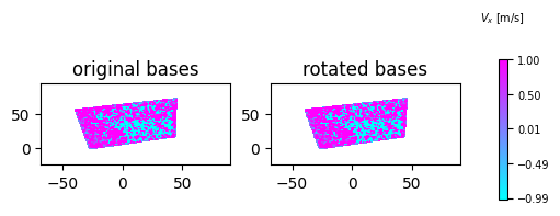
rotate_bases() function returns the same dict like data type with $V_x$ and $V_y$ projected on rotated bases. here X and Y axis are not rotated. Only the velocities are represented in new bases. So, now in new $V_x$ the x axis is aligned at $45^{\circ}$ from the horizontal.
note that the axis are not rotated. Here the velocity and any point (x,y) is projected on new bases but the velocity vector is still of point (x,y).
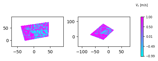
Rotate Coordinate axis
To rotate the coordinate system we can use the rotate_coordinates_degrees() function. Here input angle must be in degrees.
vmin= -1
vmax= 1
colormap='cool'

fig = plt.figure(figsize=(5,1.5))

ax1 = fig.add_subplot(121)
d1 = s1.make_data(n=25)
d1['z'] = d1['u']
ddr_davis_data.plot_contourf(ax=ax1,data=d1,
                             vmax=vmax,vmin=vmin,add_colorbar=False,colormap=colormap)

ax2 = fig.add_subplot(122)
d1['x'],d1['y'] = ddr_davis_data.rotate_coordinates_degrees(d1['x'],d1['y'],angle=45)
ddr_davis_data.plot_contourf(ax=ax2,data=d1,
                             vmax=vmax,vmin=vmin,add_colorbar=False,colormap=colormap)

plt.tight_layout()
plt.subplots_adjust(right=0.85)
ax = fig.add_axes([0.92,0.05,0.015,0.85])
ddr_davis_data.plot_colorbar(vmin=vmin,vmax=vmax,cax=ax,font_size=7,
                             colormap=colormap,roundto=2,ctitle='$V_x$ [m/s]',cticks=5)

plt.show()
Get data at a point
get_data_at_point() function gives the z value at (px,py) point from the domain.
d1 = s1.make_data(n=25)
d1['z'] = d1['u']
print(ddr_davis_data.get_data_at_point(data=d1,px=20,py=50))
-1.3974445965482185
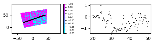
Get data at (on) the line
get_data_at_line() function returns the x,y,z values. where x,y are points on the line and z is the scalar at al (x,y) points.
d1 = s1.make_data(n=25)
d1['z'] = d1['u']

# getting data over the line
x,y,z = ddr_davis_data.get_data_at_line(data=d1,x1=-30,y1=20,x2=40,y2=50,n_points=100)

fig = plt.figure(figsize=(5,1.5))

ax1 = fig.add_subplot(121)
# plotting contour plot
ddr_davis_data.plot_contourf(data=d1,vmax=1,vmin=-1,ax=ax1,font_size=5,colormap='cool')
#plotting line over the contour plot
ax1.scatter(x,y,s=1,c='k')

ax2 = fig.add_subplot(122)
# plotting z values w.r.t y
ax2.scatter(y,z/z.max(),s=1,c='k')

plt.tight_layout()
plt.show()
Saving the data to other directory in .npy format
We need to give the name to the set and the folder path where the set will be stored. The function stores the X, Y coordinates and stores the U and V velocities image wise in subfolder.
set_foldpath = r'D:'
set_name = 'set1'
ddr_davis_data.save_set(s1,set_name=set_name,set_foldpath=set_foldpath,
                        n_start=0,n_end=3,print_info=True)
saving velocities
0
1
2
n_start and n_end specifies the starting and ending velocity files to be stored. print_info = False will disable the output shown above
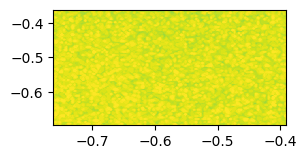
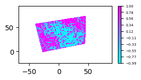
Working with local data
We can give the path to above local set, and perform all the operation with velocity datas. As we have not saved any attributes we could not retrieve it with local data.
# loading local set
ls1 = ddr_davis_data.local_set(set_name=set_name,set_foldpath=set_foldpath)

fig = plt.figure(figsize=(3,1.5))
#plotting the contour plot
d1 = ls1.make_data(n=2)
d1['z'] = d1['u']
ddr_davis_data.plot_contourf(data=d1,vmax=1,vmin=-1,colormap='cool',font_size=5)
plt.show()
we can get the length of the local set as follows
print(len(ls1))
3
Handling multiple velocitites frames
multiple velocities frames can be combined togather in single 3-D array. That array can be saved and retried later. We call this kind of multiple frames as Us and Vs.
# make 3-D array
print(ls1.get_multiple_u(0,3).shape)
(222, 295, 3)
Save the Us and Vs.
ls1.save_UVs(n_start=0,n_end=-1)
Load the Us
print(ls1.Vs.shape)
(222, 295, 3)


Download files
Download the file for your platform. If you're not sure which to choose, learn more about installing packages.
Source Distribution
Built Distribution
Hashes for ddr_davis_data-0.1.23-py3-none-any.whl
| Algorithm | Hash digest | |
|---|---|---|
| SHA256 | 14ae7f938bcc6eb1f66929317ddc4cc76ee7c37d2aa39b5eb35d116c96b79d87 |
|
| MD5 | 4f5c85884836156dca526f0b1e9f781d |
|
| BLAKE2b-256 | 9b6bd062f67a05c994876c1a142422139d6892ce8525bbf96d877281e52dfebf |


