KRATOS Multiphysics ("Kratos") is a framework for building parallel, multi-disciplinary simulation software, aiming at modularity, extensibility, and high performance. Kratos is written in C++, and counts with an extensive Python interface.

Project description
CoSimulation Application
The CoSimulation Application contains the core developments in coupling black-box solvers and other software-tools within Kratos Multiphysics.
Overview
- CoSimulation Application
List of features
-
Various features available for CoSimulation:
-
Support for MPI parallelization. This is independent of whether or not the ued solvers support/run in MPI.
-
Coupling of Kratos <=> Kratos without overhead since the same database is used and data duplication is avoided.
-
The MappingApplication is used for mapping between nonmatching grids.
Dependencies
The CoSimulation Application itself doesn't have any dependencies (except the KratosCore / KratosMPICore for serial/MPI-compilation).
For running coupled simulations the solvers to be used have to be available. Those dependencies are python-only.
The MappingApplication is required when mapping is used.
Examples
The examples can be found in the examples repository. Please also refer to the tests for examples of how the coupling can be configured. Especially the Mok-FSI and the Wall-FSI tests are very suitable for getting a basic understanding.
User Guide
This section guides users of the CoSimulationApplication to setting up and performing coupled simulations. The overall workflow is the same as what is used for most Kratos applications. It consists of the following files:
- MainKratosCoSim.py This file is to be executed with python to run the coupled simulation
- ProjectParametersCoSim.json This file contains the configuration for the coupled simulation
Setting up a coupled simulation
For running a coulpled simulation at least the two files above are required. In addition, the input for the solvers / codes participating in the coupled simulation are necessary.
The MainKratosCoSim.py file looks like this (see also here:
import KratosMultiphysics as KM
from KratosMultiphysics.CoSimulationApplication.co_simulation_analysis import CoSimulationAnalysis

"""
For user-scripting it is intended that a new class is derived
from CoSimulationAnalysis to do modifications
Check also "kratos/python_scripts/analysis-stage.py" for available methods that can be overridden
"""

parameter_file_name = "ProjectParametersCoSim.json"
with open(parameter_file_name,'r') as parameter_file:
    parameters = KM.Parameters(parameter_file.read())

simulation = CoSimulationAnalysis(parameters)
simulation.Run()
It can be executed with python:
python MainKratosCoSim.py
If the coupled simulation runs in a distributed environment (MPI) then MPI is required to launch the script
mpiexec -np 4 python MainKratosCoSim.py --using-mpi
Not the passing of the --using-mpi flag which tells Kratos that it runs in MPI.
The JSON configuration file
The configuration of the coupled simulation is written in json format, same as for the rest of Kratos.
It contains two settings:
-
problem_data: this setting contains global settings of the coupled problem.
"start_time" : 0.0,
"end_time" : 15.0,
"echo_level" : 0, // verbosity, higher values mean more output
"print_colors" : true, // use colors in the prints
"parallel_type" : "OpenMP" // or "MPI"
-
solver_settings: the settings of the coupled solver.
"type" : "coupled_solvers.gauss_seidel_weak", // type of the coupled solver, see python_scripts/coupled_solvers
"predictors" : [], // list of predictors
"num_coupling_iterations" : 10, // max number of coupling iterations, only available for strongly coupled solvers
"convergence_accelerators" : [] // list of convergence accelerators, only available for strongly coupled solvers
"convergence_criteria" : [] // list of convergence criteria, only available for strongly coupled solvers
"data_transfer_operators" : {} // map of data transfer operators (e.g. mapping)
"coupling_sequence" : [] // list specifying in which order the solvers are called
"solvers" : {} // map of solvers participating in the coupled simulation, specifying their input and interfaces
See the next section for a basic example with more explanations.
Basic FSI example
This example is the Wall FSI benchmark, see [1], chapter 7.5.3. The Kratos solvers are used to solve this problem. The input files for this example can be found here
{
    "problem_data" :
    {
        "start_time" : 0.0,
        "end_time" : 3.0,
        "echo_level" : 0, // printing no additional output
        "print_colors" : true, // using colors for prints
        "parallel_type" : "OpenMP"
    },
    "solver_settings" :
    {
        "type" : "coupled_solvers.gauss_seidel_weak", // weakly coupled simulation, no interface convergence is checked
        "echo_level" : 0, // no additional output from the coupled solver
        "predictors" : [ // using a predictor to improve the stability of the simulation
            {
                "type" : "average_value_based",
                "solver"         : "fluid",
                "data_name"      : "load"
            }
        ],
        "data_transfer_operators" : {
            "mapper" : {
                "type" : "kratos_mapping",
                "mapper_settings" : {
                    "mapper_type" : "nearest_neighbor" // using a simple mapper, see the README in the MappingApplications
                }
            }
        },
        "coupling_sequence":
        [
        {
            "name": "structure", // the structural solver comes first
            "input_data_list": [ // before solving, the following data is imported in the structural solver
                {
                    "data"              : "load",
                    "from_solver"       : "fluid",
                    "from_solver_data"  : "load", // the fluid loads are mapped onto the structure
                    "data_transfer_operator" : "mapper", // using the mapper defined above (nearest neighbor)
                    "data_transfer_operator_options" : ["swap_sign"] // in Kratos, the loads have the opposite sign, hence it has to be swapped
                }
            ],
            "output_data_list": [ // after solving, the displacements are mapped to the fluid solver
                {
                    "data"           : "disp",
                    "to_solver"      : "fluid",
                    "to_solver_data" : "disp",
                    "data_transfer_operator" : "mapper"
                }
            ]
        },
        {
            "name": "fluid", // the fluid solver solves after the structure
            "output_data_list": [],
            "input_data_list": []
        }
        ],
        "solvers" : // here we specify the solvers, their input and interfaces for CoSimulation
        {
            "fluid":
            {
                "type" : "solver_wrappers.kratos.fluid_dynamics_wrapper", // using the Kratos FluidDynamicsApplication for the fluid
                "solver_wrapper_settings" : {
                    "input_file"  : "fsi_wall/ProjectParametersCFD" // input file for the fluid solver
                },
                "data" : { // definition of interfaces used in the simulation
                    "disp" : {
                        "model_part_name" : "FluidModelPart.NoSlip2D_FSI_Interface",
                        "variable_name" : "MESH_DISPLACEMENT",
                        "dimension" : 2
                    },
                    "load" : {
                        "model_part_name" : "FluidModelPart.NoSlip2D_FSI_Interface",
                        "variable_name" : "REACTION",
                        "dimension" : 2
                    }
                }
            },
            "structure" :
            {
                "type" : "solver_wrappers.kratos.structural_mechanics_wrapper", // using the Kratos StructuralMechanicsApplication for the structure
                "solver_wrapper_settings" : {
                    "input_file"  : "fsi_wall/ProjectParametersCSM" // input file for the structural solver
                },
                "data" : { // definition of interfaces used in the simulation
                    "disp" : {
                        "model_part_name" : "Structure.GENERIC_FSI_Interface",
                        "variable_name" : "DISPLACEMENT",
                        "dimension" : 2
                    },
                    "load" : {
                        "model_part_name" : "Structure.GENERIC_FSI_Interface",
                        "variable_name" : "POINT_LOAD",
                        "dimension" : 2
                    }
                }
            }
        }
    }
}
Developer Guide
Structure of the Application
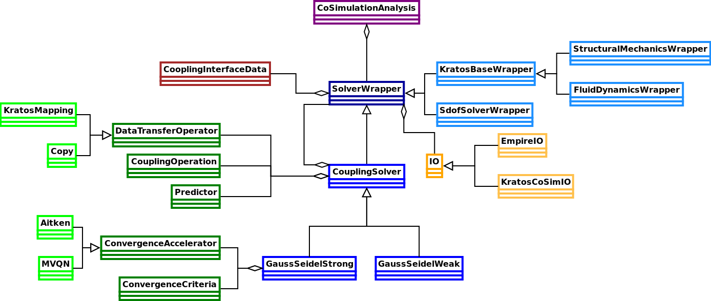
The CoSimulationApplication consists of the following main components (taken from [2]):
- SolverWrapper: Baseclass and CoSimulationApplication-interface for all solvers/codes participating in the coupled simulation, each solver/code has its own specific version.
- CoupledSolver: Implements coupling schemes such as weak/strong coupling with Gauss-Seidel/Jacobi pattern. It derives from SolverWrapper such that it can beused in nested coupled simulations.
- IO: Responsible for communicating and data exchange with external solvers/codes
- DataTransferOperator: Transfers data from one discretization to another, e.g. by use of mapping techniques
- CouplingOperation: Tool for customizing coupled simulations
- ConvergenceAccelerator: Accelerating the solution in strongly coupled simulations by use of relaxation or Quasi-Newton techniques
- ConvergenceCriteria: Checks if convergence is achieved in a strongly coupled simulation.
- Predictor: Improves the convergence by using a prediction as initial guess for the coupled solution
The following UML diagram shows the relation between these components:
Besides the functionalities listed above, the modular design of the application makes it straightforward to add a new or customized version of e.g. a ConvergenceAccelerator. It is not necessary to have those custom python scripts inside the CoSimulationApplication, it is sufficient that they are in a directory that is included in the PYTHONPATH (e.g. the working directory).
How to couple a new solver / software-tool?
The CoSimulationApplication is very modular and designed to be extended to coupling of more solvers / software-tools. This requires basically two components on the Kratos side:
The interface between the CoSimulationApplication and a solver is done with the SolverWrapper. This wrapper is specific to every solver and calls the solver-custom methods based on the input of CoSimulation.
The second component necessary is an IO. This component is used by the SolverWrapper and is responsible for the exchange of data (e.g. mesh, field-quantities, geometry etc) between the solver and the CoSimulationApplication.
In principle three different options are possible for exchanging data with CoSimulation:
- For very simple solvers IO can directly be done in python inside the SolverWrapper, which makes a separate IO superfluous (see e.g. a python-only single degree of freedom solver)
- Using the CoSimIO. This which is the preferred way of exchanging data with the CoSimulationApplication. It is currently available for C++, C, and Python. The CoSimIO is included as the KratosCoSimIO and can be used directly. Its modular and Kratos-independent design as detached interface allows for easy integration into other codes.
- Using a custom solution based on capabilities that are offered by the solver that is to be coupled.
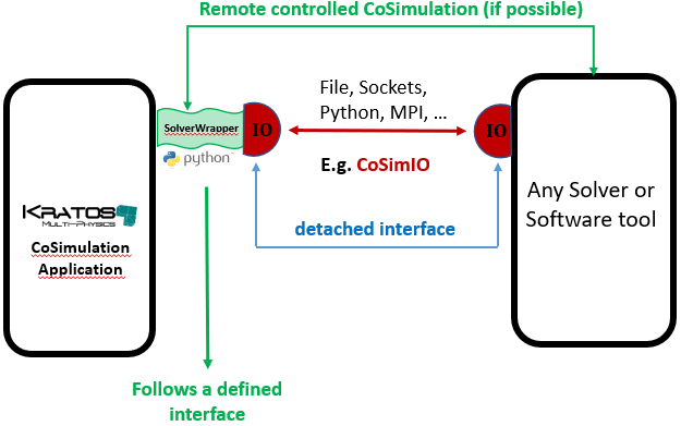
The following picture shows the interaction of these components with the CoSimulationApplication and the external solver:
Interface of SolverWrapper
The SolverWrapper is the interface in the CoSimulationApplication to all involved codes / solvers. It provides the following interface (adapted from [2]), which is also called in this order:
- Initialize: This function is called once at the beginning of the simulation, it e.g .reads the input files and prepares the internal data structures.
- The solution loop is split into the following six functions:
- AdvanceInTime: Advancing in time and preparing the data structure for the next time step.
- InitializeSolutionStep: Applying boundary conditions
- Predict: Predicting the solution of this time step to accelerate the solution.
iterate until convergence in a strongly coupled solution:- SolveSolutionStep: Solving the problem for this time step. This is the only function that can be called multiple times in an iterative (strongly coupled) solution procedure.
- FinalizeSolutionStep: Updating internals after solving this time step.
- OutputSolutionStep: Writing output at the end of a time step
- Finalize: Finalizing and cleaning up after the simulation
Each of these functions can implement functionalities to communicate with the external solver, telling it what to do. However, this is often skipped if the data exchange is used for the synchronization of the solvers. This is often done in "classical" coupling tools. I.e. the code to couple internally duplicates the coupling sequence and synchronizes with the coupling tool through the data exchange.
An example of a SolverWrapper coupled to an external solver using this approach can be found here. Only the mesh exchange is done explicitly at the beginning of the simulation, the data exchange is done inside SolveSolutionStep.
The coupled solver has to duplicate the coupling sequence, it would look e.g. like this (using CoSimIO) for a weak coupling:
# solver initializes ...

CoSimIO::ExportMesh(...) # send meshes to the CoSimulationApplication

# start solution loop
while time < end_time:
    CoSimIO::ImportData(...) # get interface data

    # solve the time step

    CoSimIO::ExportData(...) # send new data to the CoSimulationApplication
An example for an FSI problem where the structural solver of Kratos is used as an external solver can be found here. The CoSimIO is used for communicating between the CoSimulationApplication and the structural solver
While this approach is commonly used, it has the significant drawback that the coupling sequence has to be duplicated, which not only has the potential for bugs and deadlocks but also severely limits the useability when it comes to trying different coupling algorithms. Then not only the input for the CoSimulationApplication has to be changed but also the source code in the external solver!
Hence a better solution is proposed in the next section:
Remote controlled CoSimulation
A unique feature of Kratos CoSimulation (in combination with the CoSimIO) is the remotely controlled CoSimulation. The main difference to the "classical" approach which duplicates the coupling sequence in the external solver is to give the full control to CoSimulation. This is the most flexible approach from the point of CoSimulation, as then neither the coupling sequence nor any other coupling logic has to be duplicated in the external solver.
In this approach the external solver registers the functions necessary to perform coupled simulations through the CoSimIO. These are then called remotely through the CoSimulationApplication. This way any coupling algorithm can be used without changing anything in the external solver.
# defining functions to be registered
def SolveSolution()
{
    # external solver solves timestep
}

def ExportData()
{
    # external solver exports data to the CoSimulationApplication
}

# after defining the functions they can be registered in the CoSimIO:

CoSimIO::Register(SolveSolution)
CoSimIO::Register(ExportData)
# ...

# After all the functions are registered and the solver is fully initialized for CoSimulation, the Run method is called
CoSimIO::Run() # this function runs the coupled simulation. It returns only after finishing
A simple example of this can be found in the CoSimIO.
The SolverWrapper for this approach sends a small control signal in each of its functions to the external solver to tell it what to do. This could be implemented as the following:
class RemoteControlSolverWrapper(CoSimulationSolverWrapper):
    # ...
    # implement other methods as necessary
    # ...

    def InitializeSolutionStep(self):
        data_config = {
            "type"           : "control_signal",
            "control_signal" : "InitializeSolutionStep"
        }
        self.ExportData(data_config)

    def SolveSolutionStep(self):
        for data_name in self.settings["solver_wrapper_settings"]["export_data"].GetStringArray():
            # first tell the controlled solver to import data
            data_config = {
                "type"            : "control_signal",
                "control_signal"  : "ImportData",
                "data_identifier" : data_name
            }
            self.ExportData(data_config)

            # then export the data from Kratos
            data_config = {
                "type" : "coupling_interface_data",
                "interface_data" : self.GetInterfaceData(data_name)
            }
            self.ExportData(data_config)

        # now the external solver solves
        super().SolveSolutionStep()

        for data_name in self.settings["solver_wrapper_settings"]["import_data"].GetStringArray():
            # first tell the controlled solver to export data
            data_config = {
                "type"            : "control_signal",
                "control_signal"  : "ExportData",
                "data_identifier" : data_name
            }
            self.ExportData(data_config)

            # then import the data to Kratos
            data_config = {
                "type" : "coupling_interface_data",
                "interface_data" : self.GetInterfaceData(data_name)
            }
            self.ImportData(data_config)
A full example for this can be found here.
If it is possible for an external solver to implement this approach, it is recommended to use it as it is the most robust and flexible.
Nevertheless both approaches are possible with the CoSimulationApplication.
Using a solver in MPI
By default, each SolverWrapper makes use of all ranks in MPI. This can be changed if e.g. the solver that is wrapped by the SolverWrapper does not support MPI or to specify to use less rank.
The base SolverWrapper provides the _GetDataCommunicator function for this purpose. In the baseclass, the default DataCommunicator (which contains all ranks in MPI) is returned. The SolverWrapper will be instantiated on all the ranks on which this DataCommunicator is defined (i.e. on the ranks where data_communicator.IsDefinedOnThisRank() == True).
If a solver does not support MPI-parallelism then it can only run on one rank. In such cases it should return a DataCommunicator which contains only one rank. For this purpose the function KratosMultiphysics.CoSimulationApplication.utilities.data_communicator_utilities.GetRankZeroDataCommunicator can be used. Other custom solutions are also possible, see for example the structural_solver_wrapper.
References
- [1] Wall, Wolfgang A., Fluid structure interaction with stabilized finite elements, PhD Thesis, University of Stuttgart, 1999, http://dx.doi.org/10.18419/opus-127
- [2] Bucher et al., Realizing CoSimulation in and with a multiphysics framework, conference proceedings, IX International Conference on Computational Methods for Coupled Problems in Science and Engineering, 2021, https://www.scipedia.com/public/Bucher_et_al_2021a
Release history Release notifications | RSS feed


Download files
Download the file for your platform. If you're not sure which to choose, learn more about installing packages.
Source Distributions
Built Distributions
Hashes for KratosCoSimulationApplication-9.4.6-cp311-cp311-win_amd64.whl
| Algorithm | Hash digest | |
|---|---|---|
| SHA256 | 295de4da0cf7270ca36684c6368645fef103747c9900cb3ddd98d08ac88cbe87 |
|
| MD5 | 559b1b26fd0444efc2e5c21d8d146217 |
|
| BLAKE2b-256 | a2902b018a4d0cecfec58ccf9c1aa73e0623068435347a92f7e33aeded7a2453 |
Hashes for KratosCoSimulationApplication-9.4.6-cp310-cp310-win_amd64.whl
| Algorithm | Hash digest | |
|---|---|---|
| SHA256 | b37357756f0d381f6008719965f48915a5dc36b2e4820b552cc013f2e436c856 |
|
| MD5 | d10a1ad61023a045b1a2d30ae3104555 |
|
| BLAKE2b-256 | 821070199561d8965f746ebe0cb5665a70371f2a6e142bdd7df6b8a383fb4649 |
Hashes for KratosCoSimulationApplication-9.4.6-cp39-cp39-win_amd64.whl
| Algorithm | Hash digest | |
|---|---|---|
| SHA256 | 15961e4a09aa19a2c7807ab9d5705dffacee79de87893635c248e2f3dc65da34 |
|
| MD5 | 477a8bcd31096797110a363439195cb8 |
|
| BLAKE2b-256 | 75660248c850ff0b555ebf20109e1e7ab578da2ca7aec7afc89fc428898b9654 |
Hashes for KratosCoSimulationApplication-9.4.6-cp38-cp38-win_amd64.whl
| Algorithm | Hash digest | |
|---|---|---|
| SHA256 | 330e927960ac9d02d71425cec076a588d8258fa90d82cd9b139866964440dba5 |
|
| MD5 | 6d8ce009930a48abb1150f7834d5b9e2 |
|
| BLAKE2b-256 | e31db031d20629df4c959edb7be8feba2bc6d154fab74cda53d96c4ea173a6a7 |


