Feature extractor from noisy time series

Project description
light-curve processing toolbox for Python
The Python wrapper for Rust light-curve-feature and light-curve-dmdt packages which gives a collection of high-performant time-series feature extractors.


Installation
python3 -mpip install 'light-curve[full]'
full extras would install the package with all optional Python dependencies required by experimental features.
We also provide light-curve-python package which is just an "alias" to the main light-curve[full] package.
Minimum supported Python version is 3.8. We provide binary wheels via PyPi for a number of platforms and architectures, both for CPython and PyPy. We also provide binary wheels for stable CPython ABI, so the package is guaranteed to work with all future CPython3 versions.
Support matrix
| Arch \ OS | Linux glibc | Linux musl | macOS | Windows https://github.com/light-curve/light-curve-python/issues/186 |
|---|---|---|---|---|
| x86-64 | wheel (MKL) | wheel (MKL) | wheel | wheel (no Ceres, no GSL) |
| i686 | src | src | — | not tested |
| aarch64 | wheel | wheel | wheel | not tested |
| ppc64le | wheel | not tested (no Rust toolchain) | — | — |
- "wheel": binary wheel is available on pypi.org, local building is not required for the platform, the only pre-requirement is a recent
pipversion. For Linux x86-64 we provide binary wheels built with Intel MKL for better periodogram performance, which is not a default build option. For Windows x86-64 we provide wheel with no Ceres and no GSL support, which is not a default build option. - "src": the package is confirmed to be built and pass unit tests locally, but testing and package building is not supported by CI. It is required to have the GNU scientific library (GSL) v2.1+ and the Rust toolchain v1.67+ to install it via
pip install.ceres-solverandfftwmay be installed locally or built from source, in the later case you would also need C/C++ compiler andcmake. - "not tested": building from the source code is not tested, please report us building status via issue/PR/email.
Feature evaluators
Most of the classes implement various feature evaluators useful for light-curve based astrophysical source classification and characterisation.
import light_curve as lc
import numpy as np

# Time values can be non-evenly separated but must be an ascending array
n = 101
t = np.linspace(0.0, 1.0, n)
perfect_m = 1e3 * t + 1e2
err = np.sqrt(perfect_m)
m = perfect_m + np.random.normal(0, err)

# Half-amplitude of magnitude
amplitude = lc.Amplitude()
# Fraction of points beyond standard deviations from mean
beyond_std = lc.BeyondNStd(nstd=1)
# Slope, its error and reduced chi^2 of linear fit
linear_fit = lc.LinearFit()
# Feature extractor, it will evaluate all features in more efficient way
extractor = lc.Extractor(amplitude, beyond_std, linear_fit)

# Array with all 5 extracted features
result = extractor(t, m, err, sorted=True, check=False)

print('\n'.join(f"{name} = {value:.2f}" for name, value in zip(extractor.names, result)))

# Run in parallel for multiple light curves:
results = amplitude.many(
    [(t[:i], m[:i], err[:i]) for i in range(n // 2, n)],
    n_jobs=-1,
    sorted=True,
    check=False,
)
print("Amplitude of amplitude is {:.2f}".format(np.ptp(results)))
If you're confident in your inputs you could use sorted = True (t is in ascending order)
and check = False (no NaNs in inputs, no infs in t or m) for better performance.
Note that if your inputs are not valid and are not validated by
sorted=None and check=True (default values) then all kind of bad things could happen.
Print feature classes list
import light_curve as lc

print([x for x in dir(lc) if hasattr(getattr(lc, x), "names")])
Read feature docs
import light_curve as lc

help(lc.BazinFit)
Available features
See the complete list of available feature evaluators and documentation in light-curve-feature Rust crate docs.
Italic names are experimental features.
While we usually say "magnitude" and use "m" as a time-series value, some of the features are supposed to be used with flux light-curves.
The last column indicates whether the feature should be used with flux light curves only, magnitude light curves only, or any kind of light curves.
| Feature name | Description | Min data points | Features number | Flux/magnitude |
|---|---|---|---|---|
| Amplitude | Half amplitude of magnitude: $\displaystyle \frac{\max (m)-\min (m)}{2}$ |
1 | 1 | Flux or magn |
| AndersonDarlingNormal | Unbiased Anderson–Darling normality test statistic:
$\displaystyle \left( 1+\frac{4}{N} -\frac{25}{N^{2}}\right) \times$
$\times \left( -N-\frac{1}{N}\sum\limits_{i=0}^{N-1} (2i+1)\ln \Phi _{i} +(2(N-i)-1)\ln (1-\Phi _{i} )\right) ,$ where $\Phi _{i\ } \equiv \Phi (( m_{i} \ -\ \langle m\rangle ) /\sigma _{m})$ is the commutative distribution function of the standard normal distribution, $N-$ the number of observations, $\langle m\rangle -$ mean magnitude and $\sigma _{m} =\sqrt{\sum\limits_{i=0}^{N-1}( m_{i} -\langle m\rangle )^{2} /( N-1) \ }$ is the magnitude standard deviation |
4 | 1 | Flux or magn |
| BazinFit | Five fit parameters and goodness of fit (reduced $\chi ^{2}$ of the Bazin function developed for core-collapsed supernovae:
$\displaystyle f(t)=A\frac{\mathrm{e}^{-(t-t_{0} )/\tau _{fall}}}{1+\mathrm{e}^{-(t-t_{0} )/\tau _{rise}}} +B,$ where $f(t)-$ flux observation |
6 | 1 | Flux only |
| BeyondNStd | Fraction of observations beyond $n\sigma _{m}$ from the mean magnitude $\langle m\rangle $:
$\displaystyle \frac{\sum _{i} I_{|m-\langle m\rangle | >n\sigma _{m}} (m_{i} )}{N},$ where $I-$ an indicator function |
2 | 1 | Flux or magn |
| ColorOfMedian (experimental) |
Magnitude difference between medians of two bands | 2 | 1 | Magn only |
| Cusum | A range of cumulative sums:
$\displaystyle \max(S) -\min(S),$ where $S_{j} \equiv \frac{1}{N\sigma _{m}}\sum\limits _{i=0}^{j} (m_{i} -\langle m\rangle )$, $j\in \{1..N-1\}$ |
2 | 1 | Flux or magn |
| Eta | Von Neummann $\eta $:
$\displaystyle \eta \equiv \frac{1}{(N-1)\sigma _{m}^{2}}\sum\limits _{i=0}^{N-2} (m_{i+1} -m_{i} )^{2}$ |
2 | 1 | Flux or magn |
| EtaE | Modernisation of Eta for unevenly time series:
$\displaystyle \eta ^{e} \equiv \frac{(t_{N-1} -t_{0} )^{2}}{(N-1)^{3}}\frac{\sum\limits_{i=0}^{N-2}\left(\frac{m_{i+1} -m_{i}}{t_{i+1} -t_{i}}\right)^{2}}{\sigma _{m}^{2}}$ |
2 | 1 | Flux or magn |
| ExcessVariance | Measure of the variability amplitude:
$\displaystyle \frac{\sigma _{m}^{2} -\langle \delta ^{2} \rangle }{\langle m\rangle ^{2}},$ where $\langle \delta ^{2} \rangle -$ mean squared error |
2 | 1 | Flux only |
| FluxNNotDetBeforeFd (experimental) |
Number of non-detections before the first detection | 2 | 1 | Flux only |
| InterPercentileRange | $\displaystyle Q(1-p)-Q(p),$ where $Q(n)$ and $Q(d)-$ $n$-th and $d$-th quantile of magnitude sample |
1 | 1 | Flux or magn |
| Kurtosis | Excess kurtosis of magnitude:
$\displaystyle \frac{N(N+1)}{(N-1)(N-2)(N-3)}\frac{\sum _{i} (m_{i} -\langle m\rangle )^{4}}{\sigma _{m}^{2}} -3\frac{(N+1)^{2}}{(N-2)(N-3)}$ |
4 | 1 | Flux or magn |
| LinearFit | The slope, its error and reduced $\chi ^{2}$ of the light curve in the linear fit of a magnitude light curve with respect to the observation error $\{\delta _{i}\}$:
$\displaystyle m_{i} \ =\ c\ +\ \text{slope} \ t_{i} \ +\ \delta _{i} \varepsilon _{i} ,$ where $c$ is a constant, $\{\varepsilon _{i}\}$ are standard distributed random variables |
3 | 3 | Flux or magn |
| LinearTrend | The slope and its error of the light curve in the linear fit of a magnitude light curve without respect to the observation error $\{\delta _{i}\}$:
$\displaystyle m_{i} \ =\ c\ +\ \text{slope} \ t_{i} \ +\ \Sigma \varepsilon _{i} ,$ where $c$ and $\Sigma$ are constants, $\{\varepsilon _{i}\}$ are standard distributed random variables. |
2 | 2 | Flux or magn |
| MagnitudeNNotDetBeforeFd (experimental) |
Number of non-detections before the first detection | 2 | 1 | Magn only |
| MagnitudePercentageRatio | Magnitude percentage ratio:
$\displaystyle \frac{Q(1-n)-Q(n)}{Q(1-d)-Q(d)}$ |
1 | 1 | Flux or magn |
| MaximumSlope | Maximum slope between two sub-sequential observations:
$\displaystyle \max_{i=0\dotsc N-2}\left| \frac{m_{i+1} -m_{i}}{t_{i+1} -t_{i}}\right|$ |
2 | 1 | Flux or magn |
| Mean | Mean magnitude:
$\displaystyle \langle m\rangle =\frac{1}{N}\sum\limits _{i} m_{i}$ |
1 | 1 | Flux or magn |
| MeanVariance | Standard deviation to mean ratio:
$\displaystyle \frac{\sigma _{m}}{\langle m\rangle }$ |
2 | 1 | Flux only |
| Median | Median magnitude | 1 | 1 | Flux or magn |
| MedianAbsoluteDeviation | Median of the absolute value of the difference between magnitude and its median:
$\displaystyle \mathrm{Median} (|m_{i} -\mathrm{Median} (m)|)$ |
1 | 1 | Flux or magn |
| MedianBufferRangePercentage | Fraction of points within $\displaystyle \mathrm{Median} (m)\pm q\times (\max (m)-\min (m))/2$ |
1 | 1 | Flux or magn |
| OtsuSplit | Difference of subset means, standard deviation of the lower subset, standard deviation of the upper
subset and lower-to-all observation count ratio for two subsets of magnitudes obtained by Otsu's method split.
Otsu's method is used to perform automatic thresholding. The algorithm returns a single threshold that separate values into two classes. This threshold is determined by minimizing intra-class intensity variance $\sigma^2_{W}=w_0\sigma^2_0+w_1\sigma^2_1$, or equivalently, by maximizing inter-class variance $\sigma^2_{B}=w_0 w_1 (\mu_1-\mu_0)^2$. There can be more than one extremum. In this case, the algorithm returns the minimum threshold. |
2 | 4 | Flux or magn |
| PercentAmplitude | Maximum deviation of magnitude from its median:
$\displaystyle \max_{i} |m_{i} \ -\ \text{Median}( m) |$ |
1 | 1 | Flux or magn |
| PercentDifferenceMagnitudePercentile | Ratio of $p$-th inter-percentile range to the median:
$\displaystyle \frac{Q( 1-p) -Q( p)}{\text{Median}( m)}$ |
1 | 1 | Flux only |
| RainbowFit (experimental) |
Seven fit parameters and goodness of fit (reduced $\chi ^{2}$). The Rainbow method is developed and detailed here : https://arxiv.org/abs/2310.02916). This implementation is suited for transient objects. Bolometric flux and temperature functions are customizable, by default Bazin and logistic functions are used:
$\displaystyle F_{\nu}(t, \nu) = \frac{\pi\,B\left(T(t),\nu\right)}{\sigma_\mathrm{SB}\,T(t)^{4}} \times F_\mathrm{bol}(t),$ where $F_{\nu}(t, \nu)-$ flux observation at a given wavelength |
6 | 1 | Flux only |
| ReducedChi2 | Reduced $\chi ^{2}$ of magnitude measurements:
$\displaystyle \frac{1}{N-1}\sum _{i}\left(\frac{m_{i} -\overline{m}}{\delta _{i}}\right)^{2} ,$ where $\overline{m} -$ weighted mean magnitude |
2 | 1 | Flux or magn |
| Roms (Experimental) |
Robust median statistic: $\displaystyle \frac1{N-1} \sum_{i=0}^{N-1} \frac{|m_i - \mathrm{median}(m_i)|}{\sigma_i}$ |
2 | 1 | Flux or magn |
| Skew | Skewness of magnitude:
$\displaystyle \frac{N}{(N-1)(N-2)}\frac{\sum _{i} (m_{i} -\langle m\rangle )^{3}}{\sigma _{m}^{3}}$ |
3 | 1 | Flux or magn |
| StandardDeviation | Standard deviation of magnitude:
$\displaystyle \sigma _{m} \equiv \sqrt{\sum _{i} (m_{i} -\langle m\rangle )^{2} /(N-1)}$ |
2 | 1 | Flux or magn |
| StetsonK | Stetson K coefficient described light curve shape:
$\displaystyle \frac{\sum _{i}\left| \frac{m_{i} -\langle m\rangle }{\delta _{i}}\right| }{\sqrt{N\ \chi ^{2}}}$ |
2 | 1 | Flux or magn |
| VillarFit | Seven fit parameters and goodness of fit (reduced $\chi ^{2}$) of the Villar function developed for supernovae classification:
$f(t)=c+\frac{A}{1+\exp\frac{-(t-t_{0} )}{\tau _{rise}}} \times f_{fall}(t),$ $f_{fall}(t) = 1-\frac{\nu (t-t_{0} )}{\gamma }, ~~~ t< t_{0} +\gamma,$ $f_{fall}(t) = (1-\nu )\exp\frac{-(t-t_{0} -\gamma )}{\tau _{fall}}, ~~~ t \geq t_{0} + \gamma.$ where $f(t) -$ flux observation, $A, \gamma , \tau _{rise} , \tau _{fall} >0$, $\nu \in [0;1)$Here we introduce a new dimensionless parameter $\nu$ instead of the plateau slope $\beta$ from the original paper: $\nu \equiv -\beta \gamma /A$ |
8 | 8 | Flux only |
| WeightedMean | Weighted mean magnitude:
$\displaystyle \overline{m} \equiv \frac{\sum _{i} m_{i} /\delta _{i}^{2}}{\sum _{i} 1/\delta _{i}^{2}}$ |
1 | 1 | Flux or magn |
Meta-features
Meta-features can accept other feature extractors and apply them to pre-processed data.
Periodogram
This feature transforms time-series data into the Lomb-Scargle periodogram, providing an estimation of the power spectrum. The peaks argument corresponds to the number of the most significant spectral density peaks to return. For each peak, its period and "signal-to-noise" ratio are returned.
$$ \text{signal to noise of peak} \equiv \frac{P(\omega_\mathrm{peak}) - \langle P(\omega) \rangle}{\sigma_{P(\omega)}} $$
The optional features argument accepts a list of additional feature evaluators, which are applied to the power spectrum: frequency is passed as "time," power spectrum is passed as "magnitude," and no uncertainties are set.
Bins
Binning time series to bins with width $\mathrm{window}$ with respect to some $\mathrm{offset}$. $j-th$ bin boundaries are $[j \cdot \mathrm{window} + \mathrm{offset}; (j + 1) \cdot \mathrm{window} + \mathrm{offset}]$.
Binned time series is defined by $$t_j^* = (j + \frac12) \cdot \mathrm{window} + \mathrm{offset},$$ $$m_j^* = \frac{\sum{m_i / \delta_i^2}}{\sum{\delta_i^{-2}}},$$ $$\delta_j^* = \frac{N_j}{\sum{\delta_i^{-2}}},$$ where $N_j$ is a number of sampling observations and all sums are over observations inside considering bin.
Multi-band features
As of v0.8, experimental extractors (see below), support multi-band light-curve inputs.
import numpy as np
from light_curve.light_curve_py import LinearFit

t = np.arange(20, dtype=float)
m = np.arange(20, dtype=float)
sigma = np.full_like(t, 0.1)
bands = np.array(["g"] * 10 + ["r"] * 10)
feature = LinearFit(bands=["g", "r"])
values = feature(t, m, sigma, bands)
print(values)
Rainbow Fit
Rainbow (Russeil+23) is a black-body parametric model for transient light curves.
By default, it uses Bazin function as a model for bolometric flux evolution and a logistic function for the temperature evolution.
The user may customize the model by providing their own functions for bolometric flux and temperature evolution.
This example demonstrates the reconstruction of a synthetic light curve with this model.
RainbowFit requires iminuit package.
import numpy as np
from light_curve.light_curve_py import RainbowFit

def bb_nu(wave_aa, T):
    """Black-body spectral model"""
    nu = 3e10 / (wave_aa * 1e-8)
    return 2 * 6.626e-27 * nu**3 / 3e10**2 / np.expm1(6.626e-27 * nu / (1.38e-16 * T))

# Effective wavelengths in Angstrom
band_wave_aa = {"g": 4770.0, "r": 6231.0, "i": 7625.0, "z": 9134.0}

# Parameter values
reference_time = 60000.0  # time close to the peak time
# Bolometric flux model parameters
amplitude = 1.0  # bolometric flux semiamplitude, arbitrary (non-spectral) flux/luminosity units
rise_time = 5.0  # exponential growth timescale, days
fall_time = 30.0  # exponential decay timescale, days
# Temperature model parameters
Tmin = 5e3  # temperature on +infinite time, kelvins
delta_T = 10e3  # (Tmin + delta_T) is temperature on -infinite time, kelvins
k_sig = 4.0  # temperature evolution timescale, days

rng = np.random.default_rng(0)
t = np.sort(rng.uniform(reference_time - 3 * rise_time, reference_time + 3 * fall_time, 1000))
band = rng.choice(list(band_wave_aa), size=len(t))
waves = np.array([band_wave_aa[b] for b in band])

# Temperature evolution is a sigmoid function
temp = Tmin + delta_T / (1.0 + np.exp((t - reference_time) / k_sig))
# Bolometric flux evolution is the Bazin function
lum = amplitude * np.exp(-(t - reference_time) / fall_time) / (1.0 + np.exp(-(t - reference_time) / rise_time))

# Spectral flux density for each given pair of time and passband
flux = np.pi * bb_nu(waves, temp) / (5.67e-5 * temp**4) * lum
# S/N = 5 for minimum flux, scale for Poisson noise
flux_err = np.sqrt(flux * np.min(flux) / 5.0)
flux += rng.normal(0.0, flux_err)

feature = RainbowFit.from_angstrom(band_wave_aa, with_baseline=False)
values = feature(t, flux, sigma=flux_err, band=band)
print(dict(zip(feature.names, values)))
print(f"Goodness of fit: {values[-1]}")
Note, that while we don't use precise physical constant values to generate the data, RainbowFit uses CODATA 2018 values.
Experimental extractors
From the technical point of view the package consists of two parts: a wrapper for light-curve-feature Rust crate (light_curve_ext sub-package) and pure Python sub-package light_curve_py.
We use the Python implementation of feature extractors to test Rust implementation and to implement new experimental extractors.
Please note, that the Python implementation is much slower for most of the extractors and doesn't provide the same functionality as the Rust implementation.
However, the Python implementation provides some new feature extractors you can find useful.
You can manually use extractors from both implementations:
import numpy as np
from numpy.testing import assert_allclose
from light_curve.light_curve_ext import LinearTrend as RustLinearTrend
from light_curve.light_curve_py import LinearTrend as PythonLinearTrend

rust_fe = RustLinearTrend()
py_fe = PythonLinearTrend()

n = 100
t = np.sort(np.random.normal(size=n))
m = 3.14 * t - 2.16 + np.random.normal(size=n)

assert_allclose(rust_fe(t, m), py_fe(t, m),
                err_msg="Python and Rust implementations must provide the same result")
This should print a warning about experimental status of the Python class
Benchmarks
You can run all benchmarks from the Python project folder with python3 -mpytest --benchmark-enable tests/test_w_bench.py, or with slow benchmarks disabled python3 -mpytest -m "not (nobs or multi)" --benchmark-enable tests/test_w_bench.py.
Here we benchmark the Rust implementation (rust) versus feets package and our own Python implementation (lc_py) for a light curve having n=1000 observations.
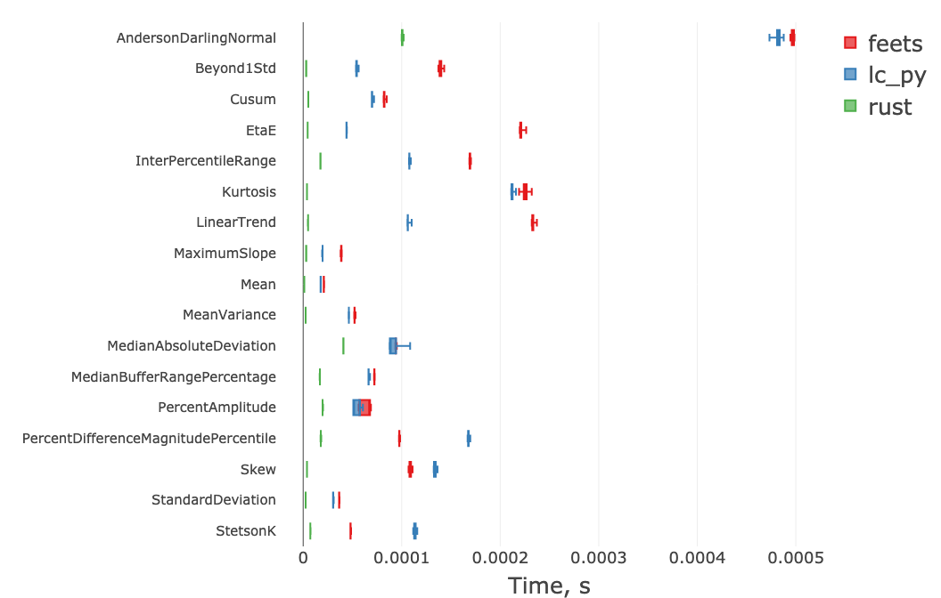
The plot shows that the Rust implementation of the package outperforms other ones by a factor of 1.5—50.
This allows to extract a large set of "cheap" features well under one ms for n=1000.
The performance of parametric fits (BazinFit and VillarFit) and Periodogram depend on their parameters, but the typical timescale of feature extraction including these features is 20—50 ms for few hundred observations.
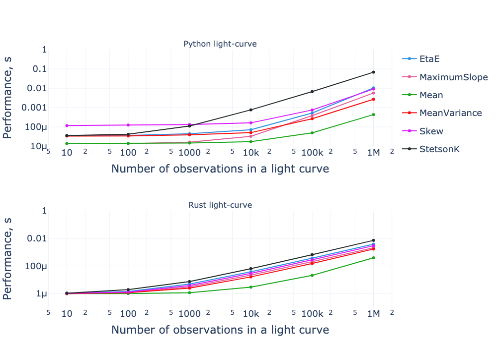
Benchmark results of several features for both the pure-Python and Rust implementations of the "light-curve" package, as a function of the number of observations in a light curve. Both the x-axis and y-axis are on a logarithmic scale.
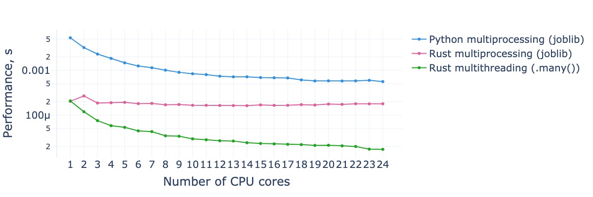
Processing time per a single light curve for extraction of features subset presented in first benchmark versus the number of CPU cores used. The dataset consists of 10,000 light curves with 1,000 observations in each.
See benchmarks' descriptions in more details in "Performant feature extraction for photometric time series".
dm-dt map
Class DmDt provides dm–dt mapper (based on Mahabal et al. 2011, Soraisam et al. 2020). It is a Python wrapper for light-curve-dmdt Rust crate.
import numpy as np
from light_curve import DmDt
from numpy.testing import assert_array_equal

dmdt = DmDt.from_borders(min_lgdt=0, max_lgdt=np.log10(3), max_abs_dm=3, lgdt_size=2, dm_size=4, norm=[])

t = np.array([0, 1, 2], dtype=np.float32)
m = np.array([0, 1, 2], dtype=np.float32)

desired = np.array(
    [
        [0, 0, 2, 0],
        [0, 0, 0, 1],
    ]
)
actual = dmdt.points(t, m)

assert_array_equal(actual, desired)
Citation
If you found this project useful for your research please cite Malanchev et al., 2021
@ARTICLE{2021MNRAS.502.5147M,
       author = {{Malanchev}, K.~L. and {Pruzhinskaya}, M.~V. and {Korolev}, V.~S. and {Aleo}, P.~D. and {Kornilov}, M.~V. and {Ishida}, E.~E.~O. and {Krushinsky}, V.~V. and {Mondon}, F. and {Sreejith}, S. and {Volnova}, A.~A. and {Belinski}, A.~A. and {Dodin}, A.~V. and {Tatarnikov}, A.~M. and {Zheltoukhov}, S.~G. and {(The SNAD Team)}},
        title = "{Anomaly detection in the Zwicky Transient Facility DR3}",
      journal = {\mnras},
     keywords = {methods: data analysis, astronomical data bases: miscellaneous, stars: variables: general, Astrophysics - Instrumentation and Methods for Astrophysics, Astrophysics - Solar and Stellar Astrophysics},
         year = 2021,
        month = apr,
       volume = {502},
       number = {4},
        pages = {5147-5175},
          doi = {10.1093/mnras/stab316},
archivePrefix = {arXiv},
       eprint = {2012.01419},
 primaryClass = {astro-ph.IM},
       adsurl = {https://ui.adsabs.harvard.edu/abs/2021MNRAS.502.5147M},
      adsnote = {Provided by the SAO/NASA Astrophysics Data System}
}
Release history Release notifications | RSS feed


Download files
Download the file for your platform. If you're not sure which to choose, learn more about installing packages.
Source Distribution
Built Distributions
Hashes for light_curve-0.9.0-pp310-pypy310_pp73-win_amd64.whl
| Algorithm | Hash digest | |
|---|---|---|
| SHA256 | 05accaaacd433aa99901a980672898083c829fe00cb8e58745569d3e47e3d640 |
|
| MD5 | 5c04f86686cb35510f9d4d66afae19f0 |
|
| BLAKE2b-256 | d77f5dac909cade07046a43d8908a30d007e8d3fac7feeb557a496cff74aa8e2 |
Hashes for light_curve-0.9.0-pp310-pypy310_pp73-manylinux_2_17_x86_64.manylinux2014_x86_64.whl
| Algorithm | Hash digest | |
|---|---|---|
| SHA256 | 34f9579afe03b7d6da6842a4768bbe0a0820213f162e81173022fb4b32b1ed27 |
|
| MD5 | 8fdbe6e3c1776d8ade0375e2bb5e5353 |
|
| BLAKE2b-256 | dd32d57faa7b0cc81674f09c2b7e96f2fbf32838328810c68c7b1a5b47b42e52 |
Hashes for light_curve-0.9.0-pp310-pypy310_pp73-manylinux_2_17_aarch64.manylinux2014_aarch64.whl
| Algorithm | Hash digest | |
|---|---|---|
| SHA256 | 575084cfe338433e42f1377eb06171a001186d89b08be070754c2ce3be1f9412 |
|
| MD5 | 30d8d6dcc42a6f7cc36864993228ca7a |
|
| BLAKE2b-256 | 5532da3c3ac339175838d2c2264a318299c2a47554b8ea45545a8d976b14ec25 |
Hashes for light_curve-0.9.0-pp310-pypy310_pp73-macosx_11_0_arm64.whl
| Algorithm | Hash digest | |
|---|---|---|
| SHA256 | 3abba2dbfdbbcabca4e161793e606ad571b8ef21e19fcce267339c4444efae2d |
|
| MD5 | b68ac92a86de9e8e43b13e809b41dd2e |
|
| BLAKE2b-256 | 3541c1ef0960720a68089cb7c9898fb30e3ea661cb25e1c8f29f77f6805da303 |
Hashes for light_curve-0.9.0-pp310-pypy310_pp73-macosx_10_9_x86_64.whl
| Algorithm | Hash digest | |
|---|---|---|
| SHA256 | c9d8a3d7fdf954a680428d85881fa1c921b94ea4ba40922dc50b543cf73572ea |
|
| MD5 | eee7dd7cfb3bf9b2d3a77869e94a5baf |
|
| BLAKE2b-256 | 076b5852de3c5bd925cda0030ae0c24e3d06c676eb2a292fd6f273eea1233fd6 |
Hashes for light_curve-0.9.0-pp39-pypy39_pp73-win_amd64.whl
| Algorithm | Hash digest | |
|---|---|---|
| SHA256 | 35c182e12e7ce9ee19898993f2596686e22c6d3debc08527a284fbca52b99b4e |
|
| MD5 | 452a7c708ece59d7117e7446d198ad5e |
|
| BLAKE2b-256 | abc0fb88192d05c107f63c94bd94b717b9e1846248632ba63b76b112f395a996 |
Hashes for light_curve-0.9.0-pp39-pypy39_pp73-manylinux_2_17_x86_64.manylinux2014_x86_64.whl
| Algorithm | Hash digest | |
|---|---|---|
| SHA256 | 0cf2ac891317b03049bbd3239f849ab3d66438a116e43f108f9591637130d545 |
|
| MD5 | 4deab5337d4091a83f15084c9e1b02ba |
|
| BLAKE2b-256 | 2ecd7b1e6f8caa141f2831df57bb01384f275f9885cc7585885f91535cc7ba25 |
Hashes for light_curve-0.9.0-pp39-pypy39_pp73-manylinux_2_17_aarch64.manylinux2014_aarch64.whl
| Algorithm | Hash digest | |
|---|---|---|
| SHA256 | fef290ad0c365d3c88bd2f2ee563e9bd5e9dc4ab358f6600152cf86934b932e5 |
|
| MD5 | cbc36e8c389b272ab7091d9df66dc814 |
|
| BLAKE2b-256 | 850cc6383542f0cb9226be217fc9bce995cf1f0d42efa9792ed818525d234775 |
Hashes for light_curve-0.9.0-pp39-pypy39_pp73-macosx_11_0_arm64.whl
| Algorithm | Hash digest | |
|---|---|---|
| SHA256 | ffc02a443255db151be094cc769188fd715522cbb96c256f897402dfa2106056 |
|
| MD5 | b03da6b8121e888f123f360ca1de04f6 |
|
| BLAKE2b-256 | 1825290d9457db009d8e4c856c87ad277246a696af98bb391ff930cbd29b63c1 |
Hashes for light_curve-0.9.0-pp39-pypy39_pp73-macosx_10_9_x86_64.whl
| Algorithm | Hash digest | |
|---|---|---|
| SHA256 | 3a217835e2d94dedd1447cbe4b24a60eb8624d7ec1ff68aa12f4dfeb9a8cc818 |
|
| MD5 | 3734a7453eec7b95b31a03501c5fa1b8 |
|
| BLAKE2b-256 | 9060da9a47f7910c2d8e3b839a79b80799b521e073b7630b151fd2daef3cea28 |
Hashes for light_curve-0.9.0-pp38-pypy38_pp73-win_amd64.whl
| Algorithm | Hash digest | |
|---|---|---|
| SHA256 | 545c60f50da83fa5eae977914f026fe4dfceeeaf11fc4098bd7e7c350169f203 |
|
| MD5 | a3feca7744ef31d87b7dd882f8c384a1 |
|
| BLAKE2b-256 | 9e1681e5e09fb7efbf00ad2d37d8a8ea2ef8078c55e2722eb439c4c7cee1188b |
Hashes for light_curve-0.9.0-pp38-pypy38_pp73-manylinux_2_17_x86_64.manylinux2014_x86_64.whl
| Algorithm | Hash digest | |
|---|---|---|
| SHA256 | bcd9671af740a4f285792060dd66c8c35761f4305f5ab38c92827bc0b2728c60 |
|
| MD5 | 32e47127ec46fd3e1d05cabbbe4124c9 |
|
| BLAKE2b-256 | 7817e6d86bcf071a4a1b9485641ddd13b658499b6935cb5af17dfd7e135ac915 |
Hashes for light_curve-0.9.0-pp38-pypy38_pp73-manylinux_2_17_aarch64.manylinux2014_aarch64.whl
| Algorithm | Hash digest | |
|---|---|---|
| SHA256 | 4ab539bc4b3a1bb998de72a57d81c79d5a1ac8a8b6066289d67dcae157535eda |
|
| MD5 | 434261bf82c55ff9846366f1d4d74b55 |
|
| BLAKE2b-256 | 04e8491299d69e2631a4f4568bdbe146d3a7e1116f6ed5bef0f4609f3f6f68c8 |
Hashes for light_curve-0.9.0-pp38-pypy38_pp73-macosx_11_0_arm64.whl
| Algorithm | Hash digest | |
|---|---|---|
| SHA256 | f5b4288804f427de4f655b9f1612d4a0d6885ee9f3d803e8fa00747c7aaccbb0 |
|
| MD5 | 440abe93cb626295f2a4ac9447eff94b |
|
| BLAKE2b-256 | 1c23f513a0d0a13a8b5ccac990e94ea14e53ac8662ac8d39fcd1b56155afd790 |
Hashes for light_curve-0.9.0-pp38-pypy38_pp73-macosx_10_9_x86_64.whl
| Algorithm | Hash digest | |
|---|---|---|
| SHA256 | 292ff67ca18cecd0fd98f4f6cbe8f4360f97930d51afa92dba0c9dd6cdb2e468 |
|
| MD5 | c5fb5b5c6fa6bb3a9d56ce3846ee7c08 |
|
| BLAKE2b-256 | 8a859e2b3ea98752e9ed888dbce71dcf856bfae298f3dfd0d121632e380c548d |
Hashes for light_curve-0.9.0-cp38-abi3-win_amd64.whl
| Algorithm | Hash digest | |
|---|---|---|
| SHA256 | 539c67050e08125a10869f1838ba010d99e859e07187adb5c6082e37d0f5b58e |
|
| MD5 | d4644b7c5253abdf2d83d58ec8ace4ea |
|
| BLAKE2b-256 | 7012c1f77c6b01026ec904998d5920fecd1772da8d0aca11c0f7c09dc1331684 |
Hashes for light_curve-0.9.0-cp38-abi3-musllinux_1_1_x86_64.whl
| Algorithm | Hash digest | |
|---|---|---|
| SHA256 | 3b42f18373246c7fe0277de2e44363bb250b2856547bdc7eb7e0a2a19fe2ce92 |
|
| MD5 | 034237f10b2ead0075f2890d14ecdc1b |
|
| BLAKE2b-256 | 5b435bbee8c4e6672742c3ac8fe4b12548e0c279addb813d139bd05e4beef1cc |
Hashes for light_curve-0.9.0-cp38-abi3-musllinux_1_1_aarch64.whl
| Algorithm | Hash digest | |
|---|---|---|
| SHA256 | bcd8c568b7c683d72ddea8db45cdee5b8be5c27ff442f30da25fea8f31b9b8d6 |
|
| MD5 | f540d92b0b21de484e421a04a2573522 |
|
| BLAKE2b-256 | 01a3b12b3335e2c405fdd57a137115a2dc6c140995f5c450c1108294d006538a |
Hashes for light_curve-0.9.0-cp38-abi3-manylinux_2_17_x86_64.manylinux2014_x86_64.whl
| Algorithm | Hash digest | |
|---|---|---|
| SHA256 | ec8377ac2c553ec118d402b7e2704857c76c302f60c6c4602b2bf6ea276da12d |
|
| MD5 | 5985de40f5dd2a0e1528b82d34d83194 |
|
| BLAKE2b-256 | 7ec81095a71491d0940c99d3ce87d8e79fb450b36a5ad522476023b307709043 |
Hashes for light_curve-0.9.0-cp38-abi3-manylinux_2_17_ppc64le.manylinux2014_ppc64le.whl
| Algorithm | Hash digest | |
|---|---|---|
| SHA256 | 78c03e073bd75580fa9d2c3dea0b76b88aed07250cdc0b7ef0f6ccfa0837ea1d |
|
| MD5 | cd98e1568132172a9bf6d90faae39fe7 |
|
| BLAKE2b-256 | f340826d046ef74c166e5c773f4c8ab4e2f520f256c6dac46ad06c54d82af70d |
Hashes for light_curve-0.9.0-cp38-abi3-manylinux_2_17_aarch64.manylinux2014_aarch64.whl
| Algorithm | Hash digest | |
|---|---|---|
| SHA256 | 1379423eeaf9c9c5e39bb0684379eadb28d197716c92e9faaba88c1da700f4f7 |
|
| MD5 | 90d6940785c4153cef23814aa71b5e84 |
|
| BLAKE2b-256 | d11195f8e8884184df96a95ec7f19ac463ab5b1e2b66f1b1d9ac80ef0d6bc409 |
Hashes for light_curve-0.9.0-cp38-abi3-macosx_11_0_arm64.whl
| Algorithm | Hash digest | |
|---|---|---|
| SHA256 | aa72941f1c8e3c31102ed284bbf9852d996be99864a2d6756eca4ef65f8e419a |
|
| MD5 | 176859d261cabf56a8b567afa70eba6a |
|
| BLAKE2b-256 | c18d52e1a0b2584de24911fed8621bbc1d61b2efbd735c94df8f6016a2c07ba7 |
Hashes for light_curve-0.9.0-cp38-abi3-macosx_10_9_x86_64.whl
| Algorithm | Hash digest | |
|---|---|---|
| SHA256 | 802a32b3edae6cea9129023b8c062c7d331464d7c0a87fde802028973e823445 |
|
| MD5 | e06645b987a83df7dfec050ea19a2ece |
|
| BLAKE2b-256 | ec4f8f25d85f6cc4e1377fb3cd13f7b9d30c289384c579602f8e7ffc7691d511 |


