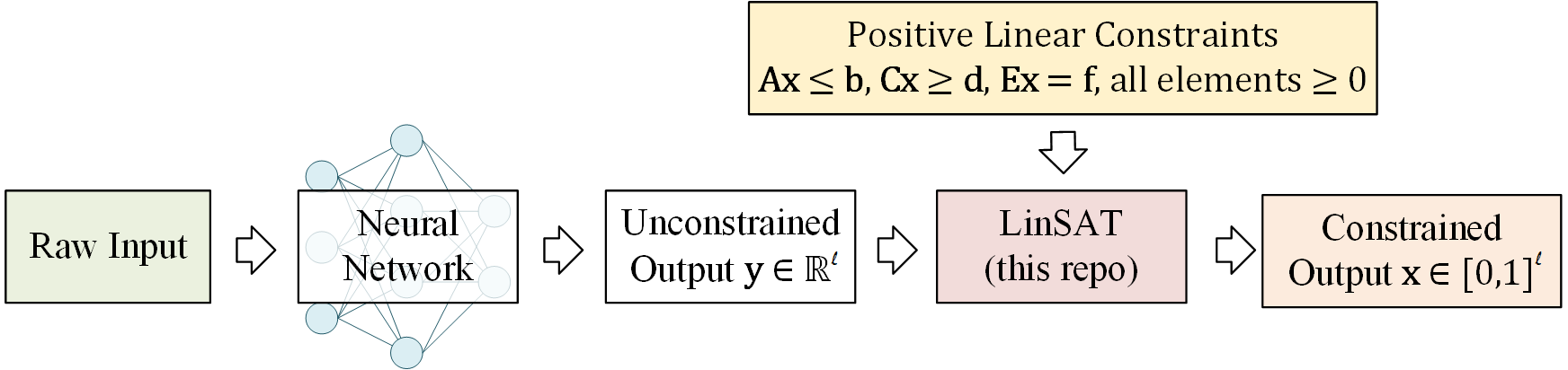
LinSATNet offers a neural network layer to enforce the satisfiability of positive linear constraints to the output of neural networks. The gradient through the layer is exactly computed. This package now works with PyTorch.

Project description
LinSATNet
This is the official implementation of our ICML 2023 paper "LinSATNet: The Positive Linear Satisfiability Neural Networks".
With LinSATNet, you can enforce the satisfiability of general positive linear constraints to the output of neural networks.

v0.1.1! The forward and backward should be identical to the dense
version, but the sparse version is expected to be more efficient in time and GPU memory. Upgrade by
pip install --upgrade linsatnet
The LinSAT layer is fully differentiable, and the gradients are exactly computed. Our implementation now supports PyTorch.
You can install it by
pip install linsatnet
And get started by
from LinSATNet import linsat_layer
A Quick Example
There is a quick example if you run LinSATNet/linsat.py directly. In this
example, the doubly-stochastic constraint is enforced for 3x3 variables.
To run the example, first clone the repo:
git clone https://github.com/Thinklab-SJTU/LinSATNet.git
Go into the repo, and run the example code:
cd LinSATNet
python LinSATNet/linsat.py
In this example, we try to enforce doubly-stochastic constraint to a 3x3 matrix. The doubly-stochastic constraint means that all rows and columns of the matrix should sum to 1.
The 3x3 matrix is flattened into a vector, and the following positive linear constraints are considered (for $\mathbf{E}\mathbf{x}=\mathbf{f}$):
E = torch.tensor(
    [[1, 1, 1, 0, 0, 0, 0, 0, 0],
     [0, 0, 0, 1, 1, 1, 0, 0, 0],
     [0, 0, 0, 0, 0, 0, 1, 1, 1],
     [1, 0, 0, 1, 0, 0, 1, 0, 0],
     [0, 1, 0, 0, 1, 0, 0, 1, 0],
     [0, 0, 1, 0, 0, 1, 0, 0, 1]], dtype=torch.float32
)
f = torch.tensor([1, 1, 1, 1, 1, 1], dtype=torch.float32)
We randomly init w and regard it as the output of some neural networks:
w = torch.rand(9) # w could be the output of neural network
w = w.requires_grad_(True)
We also have a "ground-truth target" for the output of linsat_layer, which
is an diagonal matrix in this example:
x_gt = torch.tensor(
    [1, 0, 0,
     0, 1, 0,
     0, 0, 1], dtype=torch.float32
)
The forward/backward passes of LinSAT follow the standard PyTorch style and are readily integrated into existing deep learning pipelines.
The forward pass:
linsat_outp = linsat_layer(w, E=E, f=f, tau=0.1, max_iter=10, dummy_val=0)
The backward pass:
loss = ((linsat_outp - x_gt) ** 2).sum()
loss.backward()
You can also set E as a sparse matrix to improve the time & memory efficiency
(especially for large-sized input):
linsat_outp = linsat_layer(w, E=E.to_sparse(), f=f, tau=0.1, max_iter=10, dummy_val=0)
We can also do gradient-based optimization over w to make the output of
linsat_layer closer to x_gt. This is what's happening when you train a
neural network.
niters = 10
opt = torch.optim.SGD([w], lr=0.1, momentum=0.9)
for i in range(niters):
    x = linsat_layer(w, E=E, f=f, tau=0.1, max_iter=10, dummy_val=0)
    cv = torch.matmul(E, x.t()).t() - f.unsqueeze(0)
    loss = ((x - x_gt) ** 2).sum()
    loss.backward()
    opt.step()
    opt.zero_grad()
    print(f'{i}/{niters}\n'
          f'  underlying obj={torch.sum(w * x)},\n'
          f'  loss={loss},\n'
          f'  sum(constraint violation)={torch.sum(cv[cv > 0])},\n'
          f'  x={x},\n'
          f'  constraint violation={cv}')
And you are likely to see the loss decreasing during the gradient steps.
API Reference
To use LinSATNet in your own project, make sure you have the package installed:
pip install linsatnet
and import the pacakge at the beginning of your code:
from LinSATNet import linsat_layer, init_constraints
The linsat_layer function
LinSATNet.linsat_layer(x, A=None, b=None, C=None, d=None, E=None, f=None, constr_dict=None, tau=0.05, max_iter=100, dummy_val=0, mode='v2', grouped=True, no_warning=False) [source]
LinSAT layer enforces positive linear constraints to the input x and
projects it with the constraints
$$\mathbf{A} \mathbf{x} <= \mathbf{b}, \mathbf{C} \mathbf{x} >= \mathbf{d}, \mathbf{E} \mathbf{x} = \mathbf{f}$$
and all elements in $\mathbf{A}, \mathbf{b}, \mathbf{C}, \mathbf{d}, \mathbf{E}, \mathbf{f}$ must be non-negative.
Parameters:
x: PyTorch tensor of size ($n_v$), it can optionally have a batch size ($b \times n_v$)A,C,E: PyTorch tensor of size ($n_c \times n_v$), constraint matrix on the left hand sideb,d,f: PyTorch tensor of size ($n_c$), constraint vector on the right hand sideconstr_dict: a dictionary with initialized constraint information, which is the output of the functionLinSATNet.init_constraints. Specifying this variable could avoid re-initializing the constraints for the same constraints and improve the efficiencytau: (default=0.05) parameter to control the discreteness of the projection. Smaller value leads to more discrete (harder) results, larger value leads to more continuous (softer) results.max_iter: (default=100) max number of iterationsdummy_val: (default=0) the value of dummy variables appended to the input vectormode: (default='v2') LinSAT kernel implementation.v1is the one came with the ICML paper,v2is the improved version with (usually) better efficiencygrouped: (default=True) group non-overlapping constraints in one operation for better efficiencyno_warning: (default=False) turn off warning message
return: PyTorch tensor of size ($n_v$) or ($b \times n_v$), the projected variables
Notations:
- $b$ means the batch size.
- $n_c$ means the number of constraints ($\mathbf{A}$, $\mathbf{C}$, $\mathbf{E}$ may have different $n_c$)
- $n_v$ means the number of variables
Some practical notes
- You must ensure that your input constraints have a non-empty feasible space.
Otherwise,
linsat_layerwill not converge. It is also worth noting thatxis in the range of[0, 1], and you may add a multiplier to scale it. - You may tune the value of
taufor your specific tasks. Monitor the output of LinSAT so that the "smoothness" of the output meets your task. Reasonable choices oftaumay range from1e-4to100in our experience. - Be careful of potential numerical issues. Sometimes
A x <= 1does not work, butA x <= 0.999works. - The input vector
xmay have a batch dimension, but the constraints can not have a batch dimension. The constraints should be consistent for all data in one batch. - Input constraints as sparse tensors can usually help you save GPU memory. When
working with sparse constraints,
A,C,Eshould betorch.sparse_coo_tensor, andb,d,fshould be dense tensors.
Citation
If you find our paper/code useful in your research, please cite
@inproceedings{WangICML23,
  title={{LinSATNet}: The Positive Linear Satisfiability Neural Networks},
  author={Wang, Runzhong and Zhang, Yunhao and Guo, Ziao and Chen, Tianyi and Yang, Xiaokang and Yan, Junchi},
  booktitle={International Conference on Machine Learning (ICML)},
  year={2023}
}
Release history Release notifications | RSS feed


Download files
Download the file for your platform. If you're not sure which to choose, learn more about installing packages.
Source Distribution
Built Distribution
Hashes for LinSATNet-0.1.3-py3-none-any.whl
| Algorithm | Hash digest | |
|---|---|---|
| SHA256 | 2d0023dc4a2c42759b6fc3dfd2a68784759b7f7b7a71d8424d101899b0008e33 |
|
| MD5 | 264c7b02178c2738a1937471230ca575 |
|
| BLAKE2b-256 | 38706a2af7c8012c2cd7107fe033b86145badd2b444bed7798b3ae443cc16bd7 |


