Extending scikit-learn with various useful things.

Project description


scikit-bonus
This is a package with scikit-learn - compatible transformers, classifiers and regressors that I find useful.
Give it a try with a simple pip install scikit-bonus! You can find the documentation on https://garve.github.io/scikit-bonus.
Special linear regressors
This module contains linear regressors for special use-cases, for example
- the
LADRegressionwhich optimizes for the absolute mean deviation (error) instead of the mean squared error and - the
ImbalancedLinearRegressionthat lets you punish over and under estimations of the model differently.
Since a picture says more than a thousand words:
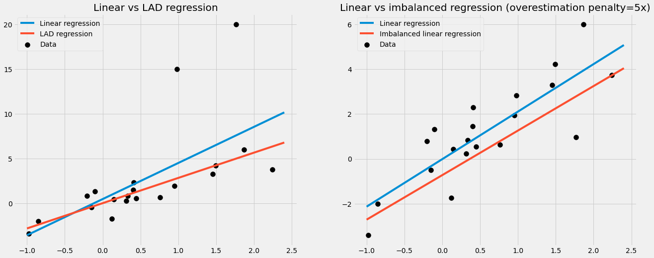
In the right picture, an imbalanced linear regression was trained to punish overestimations by the model 5 times as high as under estimations. That's why it makes sense that the imbalanced regression line is lower: the model is more afraid of overestimate the true labels.
The time module
The time module contains transformers for dealing with time series in
a simple-to-understand way.
Most of them assume the input to be a pandas
dataframe with a DatetimeIndex
with a fixed frequency, for example created via
pd.date_range(start="2020-12-12", periods=5, freq="d").
Let us see two examples of what this module provides for you.
SimpleTimeFeatures
Very often, you don't need to use complicated models such as an RNN or ARIMA. It is often sufficient to just extract some simple date features from the DatetimeIndex and run a simple, even linear regression. These features can be the hour, the day of the week, the week of the year, or the month, among others.
Let us look at an example:
import pandas as pd
from skbonus.pandas.time import SimpleTimeFeatures

data = pd.DataFrame(
    {"X_1": range(10)},
    index=pd.date_range(start="2020-01-01", periods=10, freq="d")
)

tfa = SimpleTimeFeatures(day_of_month=True, month=True, year=True)
tfa.fit(data)
print(tfa.transform(data))

------------------------------------------
OUTPUT:

            X_1  day_of_month  month  year
2020-01-01    0             1      1  2020
2020-01-02    1             2      1  2020
2020-01-03    2             3      1  2020
2020-01-04    3             4      1  2020
2020-01-05    4             5      1  2020
2020-01-06    5             6      1  2020
2020-01-07    6             7      1  2020
2020-01-08    7             8      1  2020
2020-01-09    8             9      1  2020
2020-01-10    9            10      1  2020
The SimpleTimeFeatures has many more built-in features. The full list is
- second
- minute
- hour
- day_of_week
- day_of_month
- day_of_year
- week_of_month
- week_of_year
- month
- year
You can work with these features directly, but of course, you can utilize scikit-bonus to further process these features, such as with a OneHotEncoderWithNames, a thin wrapper around scikit-learn's OneHotEncoder. Another way to post-process these features is using the CyclicalEncoder of scikit-bonus.
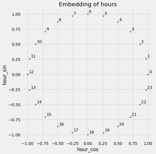
CyclicalEncoder
In short, this encoder takes a single cyclic feature such as most time features (except for year) and converts it into a two-dimensional feature with the property that close points in time are close in the encoded space.
Consider hours for example: A model working with hours in the form 0 - 23 cannot know that 0 and 23 are actually close together in time. The CyclicalEncoder arranges the hours in the way you know it from a normal, analog, round clock.
In code:
import pandas as pd
from skbonus.preprocessing.time import CyclicalEncoder

data = pd.DataFrame({"hour": range(24)})

ce = CyclicalEncoder(cycles=[(0, 23)])
ce.fit(data)
print(ce.transform(data.query("hour in [22, 23, 0, 1, 2]")))

------------------------------------------
OUTPUT:

[[ 1.          0.        ]
 [ 0.96592583  0.25881905]
 [ 0.8660254   0.5       ]
 [ 0.8660254  -0.5       ]
 [ 0.96592583 -0.25881905]]
Note that the hours 0 and 23 are as close together as 0 and 1.
Air Passengers
Let us check out the famous air passenger example:
from sktime.datasets import load_airline

data_raw = load_airline()
print(data_raw)
This yields the pandas series
Period
1949-01    112.0
1949-02    118.0
1949-03    132.0
1949-04    129.0
1949-05    121.0
           ...
1960-08    606.0
1960-09    508.0
1960-10    461.0
1960-11    390.0
1960-12    432.0
Freq: M, Name: Number of airline passengers, Length: 144, dtype: float64
While the index of this series looks fine, it's actually a PeriodIndex which scikit-bonus cannot deal with so far. Also, it's a series and not a dataframe.
We can address both problems via
data = (
    data_raw
    .to_frame() # convert to dataframe
    .set_index(data_raw.index.to_timestamp()) # overwrite index with a DatetimeIndex
)
Let us create the dataset in the scikit-learn-typical X, y form and split it into a train and test set. Note that we do not do a random split since we deal with a time series.
If there is a date from the test set between two dates that are in the training set, it might leak information about the label of the test set.
So, let us use the first 100 dates as the training set, and the remaining 44 are the test set.
X = data.drop(columns=["Number of airline passengers"])
y = data["Number of airline passengers"]

X_train = X.iloc[:100]
X_test = X.iloc[100:]
y_train = y[:100]
y_test = y[100:]
Before we continue, let us take a look at the time series.
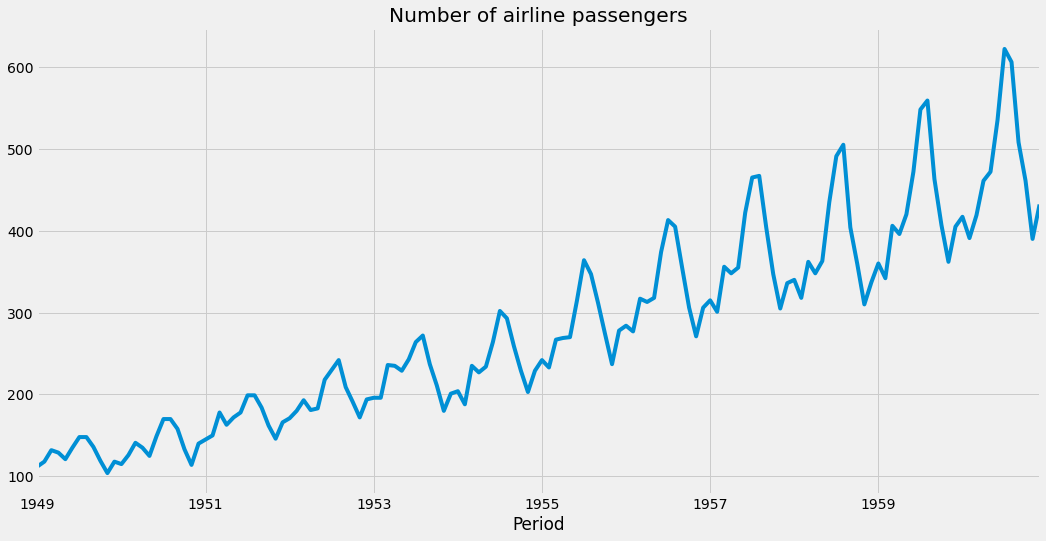
We can see that it has
- an increasing amplitude
- a seasonal pattern
- an upward trend
We want to cover these properties with the following approach:
- apply the logarithm on the data
- extract the month from the DatetimeIndex using scikit-bonus' SimpleTimeFeatures
- Add a linear trend using scikit-bonus' PowerTrend
Putting everything together in a pipeline looks like this:
from skbonus.pandas.time import SimpleTimeFeatures, PowerTrend
from skbonus.pandas.preprocessing import OneHotEncoderWithNames
from sklearn.linear_model import LinearRegression
from sklearn.compose import TransformedTargetRegressor, make_column_transformer
from sklearn.pipeline import make_pipeline
ct = make_column_transformer(
(OneHotEncoderWithNames(), ["month"]),
remainder="passthrough"
)
pre = make_pipeline(
SimpleTimeFeatures(month=True),
PowerTrend(power=0.92727), # via hyper parameter optimization
ct,
TransformedTargetRegressor(
regressor=LinearRegression(),
func=np.log, # log the data
inverse_func=np.exp # transform it back
)
)
pre.fit(X_train, y_train)
pre.score(X_test, y_test)
---------------------
OUTPUT:
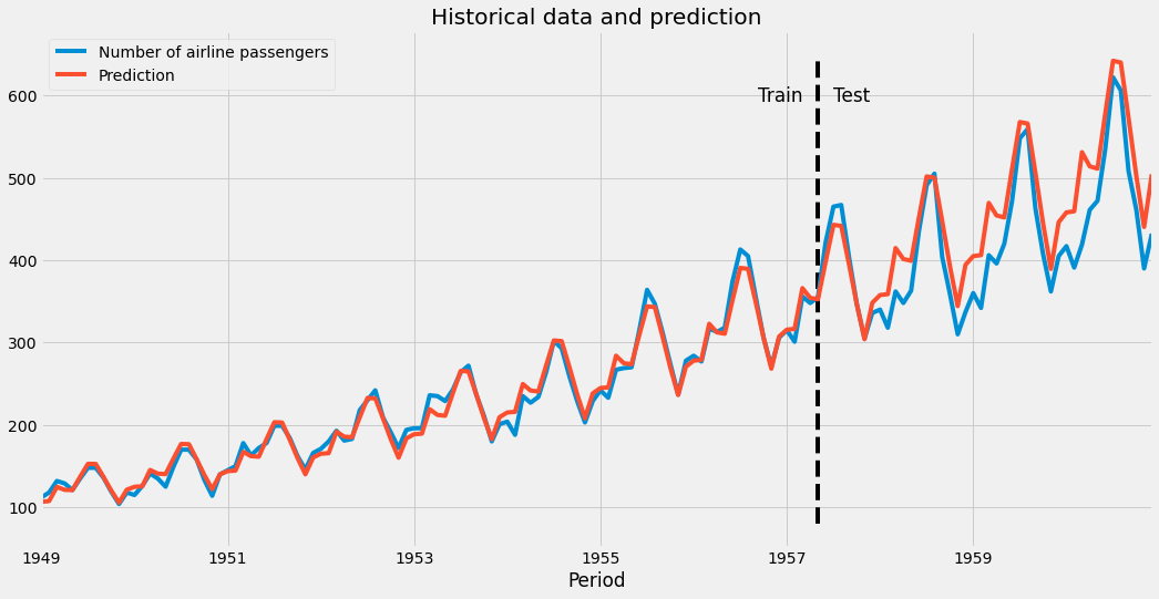
0.6843610111874758
Quite decent for such a simple model! Our predictions look like this:
Release history Release notifications | RSS feed


Download files
Download the file for your platform. If you're not sure which to choose, learn more about installing packages.
Source Distributions
Built Distribution
Hashes for scikit_bonus-0.1.12-py3-none-any.whl
| Algorithm | Hash digest | |
|---|---|---|
| SHA256 | 50a34592c3944afaf59a177ec7aa71054a7f10cbf6c3543acd75bb2624344326 |
|
| MD5 | 5839033621444f457ed13516343e5089 |
|
| BLAKE2b-256 | 28a5402194ada1f82eb70a0c39fad05d8bdc9dac0b0e50af1ab6b3467dd26afd |


