Create and visualize Lindenmayer systems

Project description
lsys
Create and visualize lindenmayer systems.


Getting Started
lsys is a library for creating Lindenmayer systems inspired by Flake's The Computational Beauty of Nature.
The graphics in that book are extraordinary, and this little tool helps make similar graphics with matplotlib.
From the text, an L-system consists of a special seed, an axiom, from which the fractal growth follows according to certain production rules. For example, if 'F' is move foward and "+-" are left and right, we can make the well-known Dragon curve using the following axiom and production rules:
import matplotlib.pyplot as plt

import lsys
from lsys import Lsys, Fractal


axiom = "FX"
rule = {"X": "X+YF+", "Y": "-FX-Y"}

dragon = Lsys(axiom=axiom, rule=rule, ignore="XY")

for depth in range(4):
    dragon.depth = depth
    print(depth, dragon.string)
0 FX
1 FX+YF+
2 FX+YF++-FX-YF+
3 FX+YF++-FX-YF++-FX+YF+--FX-YF+
Note how the production rules expand on the axiom, expanding it at each depth according to the characters in the string. If we interpret the string as a turtle graphics instruction set and move forward each time we see 'F' and left or right each time we see '-' or '+' we can visualize the curve.
dragon.depth = 3
_ = dragon.plot(lw=5)

dragon.depth = 12
_ = dragon.plot(lw=1)
The Lsys object exposes multiple options for interacting with the results of the L-system expansion, including the xy coordinates, depths of each segment, and even functions for forming bezier curves to transition between vertices of the fractal.
This allows for easier visulaization of the path that the fractal takes when the vertices of the expansion start to overlap.
For the Dragon curve, this can lead to some satisfying results.
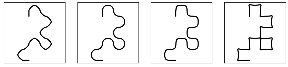
dragon.depth = 4

fig, axes = plt.subplots(1, 2, figsize=(6, 3))

_ = dragon.plot(ax=axes[0], lw=5, c="k", square=True)
_ = dragon.plot(ax=axes[1], lw=5, square=True, as_bezier=True)
dragon.depth = 12
_ = dragon.plot(lw=1, as_bezier=True)
It's also possible to use a colormap to show the path.
The most efficient way to do this in matplotlib uses the PathCollection with each segment as a cubic bezier curve.
By default, the curves are approximately circular, but the weight of the control points can be adjusted.
dragon.depth = 4
fig, axes = plt.subplots(1, 4, figsize=(12, 5))

for ax, weight in zip(axes, [0.3, None, 0.8, 1.5]):
    _ = dragon.plot_bezier(ax=ax, bezier_weight=weight, lw=3, square=True)
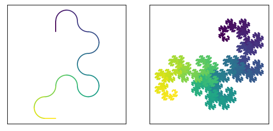
The bezier functionality also allows for applying a color map, which is useful for uncovering how the path unfolds, especially for large depths of the fractal
fig, axes = plt.subplots(1, 2, figsize=(6, 3))

for ax, depth in zip(axes, [4, 13]):
    dragon.depth = depth
    _ = dragon.plot_bezier(ax=ax, lw=1.5, square=True, cmap="viridis")
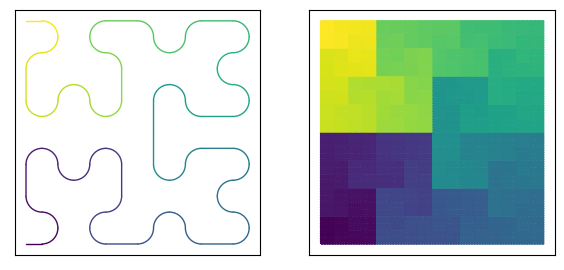
hilbert = Lsys(**Fractal["Hilbert"])
fig, axes = plt.subplots(1, 2, figsize=(6, 3))

for ax, depth in zip(axes, [2, 7]):
    hilbert.depth = depth
    _ = hilbert.plot_bezier(ax=ax, lw=1, square=True, cmap="viridis")
The plotting features allow for a fast and deep rendering, as well as a slower rendering algorithm that allows the user to choose the number of bezier segments per segment in the line collection. This feature allows for either high fidelity (many segments) color rendering of the smooth bezier path, or low fidelity
dragon.depth = 4

fig, axes = plt.subplots(1, 5, figsize=(15, 3))

# Default renderer for bezier, peak bezier rendering performance for colormapped renderings, noticably
# low color fidelity per curve at low fractal depths
_ = dragon.plot_bezier(ax=axes[0], lw=10, square=True, cmap="magma")

# line collection with custom n-segments, slower rendering due to many lines, customizably
# high or low color fidelity per curve
_ = dragon.plot_bezier(
    ax=axes[1], lw=10, square=True, cmap="magma", segs=10, as_lc=True
)
_ = dragon.plot_bezier(ax=axes[2], lw=10, square=True, cmap="magma", segs=1, as_lc=True)

# High rendering performance, but rendered as single path with a single color.
# This is the default render if `segs` is not None and `as_lc` is not set True (default is False)
_ = dragon.plot_bezier(ax=axes[3], lw=10, square=True, segs=10, c="C2")
_ = dragon.plot_bezier(ax=axes[4], lw=10, square=True, segs=1, c="C0")

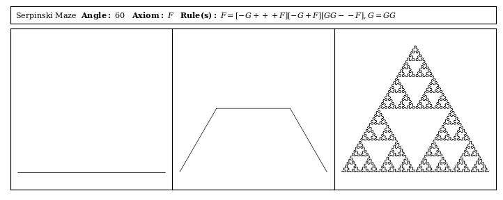
Exploring Other Fractals
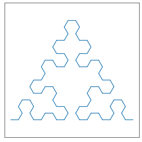
Serpinski_Maze = {
    "name": "Serpinski Maze",
    "axiom": "F",
    "rule": "F=[-G+++F][-G+F][GG--F],G=GG",
    "da": 60,
    "a0": 0,
    "ds": 0.5,
    "depth": 4,
}

_ = Lsys(**Serpinski_Maze).plot()
def build_computational_beauty_of_nature_plot(lsystem: Lsys, depths=None, **fig_kwargs):

    if depths is None:
        depths = [0, 1, 4]

    assert len(depths) == 3, "`depths` must be length 3"

    fig_kwargs_default = dict(
        figsize=(9, 3.5),
        gridspec_kw={"wspace": 0, "hspace": 0.01, "height_ratios": [1, 10]},
    )

    fig_kwargs_default.update(fig_kwargs)

    lsystem.depth = depths[-1]
    xlim, ylim = lsys.viz.get_coord_lims(lsystem.coords, pad=5, square=True)

    fig, axes = plt.subplot_mosaic([[1, 1, 1], [2, 3, 4]], **fig_kwargs_default)

    for i, (l, ax) in enumerate(axes.items()):
        ax.set_xticks([])
        ax.set_yticks([])

    plot_text = (
        f"{lsystem.name}  "
        r"$\bf{Angle:}$ "
        f"{lsystem.da}   "
        r"$\bf{Axiom:}$ "
        r"$\it{" + lsystem.axiom + "}$   "
        r"$\bf{Rule(s):}$ "
        r"$\it{" + lsystem.rule + "}$   "
    )

    axes[1].text(
        0.01,
        0.5,
        plot_text,
        math_fontfamily="dejavuserif",
        fontfamily="serif",
        va="center",
        size=8,
    )

    plot_axes = [axes[i] for i in [2, 3, 4]]

    for ax, depth in zip(plot_axes, depths):
        lsystem.depth = depth
        lsystem.plot(ax=ax, lw=0.5, c="k")

        ax.set_xlim(xlim)
        ax.set_ylim(ylim)
        _ = ax.set_aspect("equal")

    return fig, axes
_ = build_computational_beauty_of_nature_plot(
    lsystem=Lsys(**Serpinski_Maze),
    depths=[0, 1, 7],
)
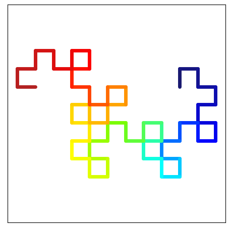
Additional Rendering Options
The lsys library has a few rendering helpers, like one to build up custom color maps.
Here is one of my favorites:
dragon.depth = 6
cmap = lsys.viz.make_colormap(
    [
        "midnightblue",
        "blue",
        "cyan",
        "lawngreen",
        "yellow",
        "orange",
        "red",
        "firebrick",
    ]
)
_ = dragon.plot(lw=5, square=True, as_lc=True, cmap=cmap)
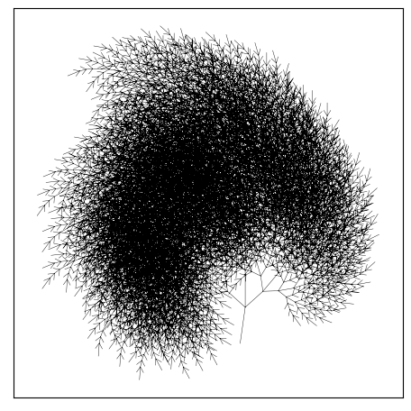
This colormap helper can also assist with non-hideous abuses of colormaps, like when rendering a tree-like fractal.
Fractal["Tree2"]
{'depth': 4,
 'axiom': 'F',
 'rule': 'F = |[5+F][7-F]-|[4+F][6-F]-|[3+F][5-F]-|F',
 'da': 8,
 'a0': 82,
 'ds': 0.65}
tree = Lsys(**Fractal["Tree2"])
tree.depth = 5
_ = tree.plot(c="k", lw=0.3)
We can add some color by creating a colormap that transitions from browns to greens.
cmap = lsys.viz.make_colormap(
    ["saddlebrown", "saddlebrown", "sienna", "darkgreen", "yellowgreen"]
)
_ = tree.plot(as_lc=True, cmap=cmap)
This has rendered each of our line segments in the order that the string expansion of the axiom and rules defined. It's interesting to see when each part of the tree appears in the linear order of the string expansion, but it's not really tree-like and it's not yet 'non-hideous'. We can do better.
The Lsys objects store an array of the depth of each line segment.
This depth changes when the string expansion algorithm encounters a push character ("[") or a pop character ("]").
Not every fractal has push and pop characters, but for those that do, the depth array can be useful for rendering.
cmap = lsys.viz.make_colormap(
    ["saddlebrown", "saddlebrown", "sienna", "darkgreen", "yellowgreen"]
)
_ = tree.plot(as_lc=True, array=tree.depths, cmap=cmap)
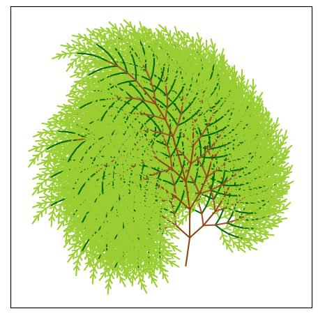
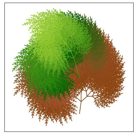
This is somewhat closer to the intention. Now the colors are mapped correctly to each segments fractal depth and trunk/stem segments are brown while branch and leaf segments are green. Even still, we can do better.
If we render each depth in separate line collections and in order of depth rather than in order of the string expansion, we can improve our tree-like rendering.
import numpy
from matplotlib.collections import LineCollection
tree = Lsys(**Fractal["Tree2"])

for d in range(5):
    tree.depth = d
    print(set(tree.depths))
{0}
{1}
{1, 2}
{1, 2, 3}
{1, 2, 3, 4}
Sidenote: The string expansion rules for this fractal nuke the first depth (0th) on the first expansion with the "|[" character combo. We'll account for this when we render things.
tree = Lsys(**Fractal["Tree2"])
tree.depth = 5

fig, ax = plt.subplots(figsize=(7, 7))
cmap = lsys.viz.make_colormap(
    ["saddlebrown", "saddlebrown", "sienna", "darkgreen", "yellowgreen"]
)
_ = lsys.viz.pretty_format_ax(ax=ax, coords=tree.coords)

for depth in range(tree.depth):
    # each depth will have a single value for color, lineweight, and alpha.
    color = cmap((depth + 1) / tree.depth)
    lw = 10 / (depth + 2)
    alpha = 0.5 if depth + 2 >= tree.depth else 1

    lc = LineCollection(
        tree.coords[tree.depths == (depth + 1)],
        color=color,
        lw=lw,
        alpha=alpha,
        capstyle="round",
    )

    ax.add_collection(lc)
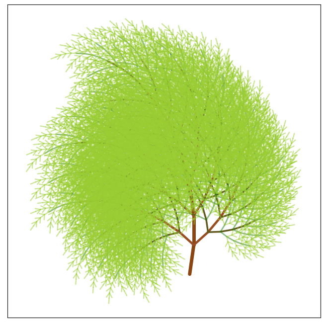
Rendering Sequences
It can be fun to see how each of these fractals evolve, so here are a few examples of watching how the dragon fractal 'winds' itself up.
d = Lsys(**Fractal["Dragon"])
d.a0 = 0
depths = range(12)
rows = int(numpy.ceil(len(depths) / 4))
fig_width = 12
fig_height = int(fig_width / 4 * rows)
fig, axes = plt.subplots(rows, 4, figsize=(fig_width, fig_height))

for ax, depth in zip(axes.flatten(), depths):
    d.depth = depth
    ax = d.plot_bezier(ax=ax, lw=3, square=True, cmap="viridis", segs=10)
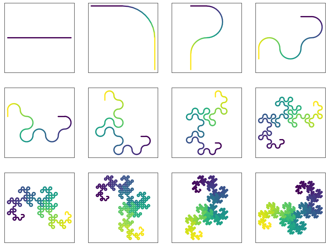
Sequences like this lend themselves nicely to creating animations. Here's one showing another way this fractal 'winds' in on itself. For this one to work, we've got to do some math to scale each plot and change the start angle for each depth.
from matplotlib import animation
from matplotlib import rc

rc("animation", html="html5")
d = Lsys(**Fractal["Dragon"])
# The difference between depth 0 and depth 1 shows where the sqrt(2) comes from
# as the line shifts into a right triangle.
d.ds = 1 / numpy.sqrt(2)

# start with bearing to the right and find all bearings for our depths
# by adding 45 deg to the start bearing for each depth
d.a0 = 0
depths = list(range(12))
a0s = [d.a0 + 45 * i for i in depths]

fig, ax = plt.subplots(figsize=(6, 6))

# set axes lims to enclose the final wound up dragon using a helper function
# that takes the coordinates of the fractal.
d.depth = depths[-1]
d.a0 = a0s[-1]
ax = lsys.viz.pretty_format_ax(ax, coords=d.coords, pad=10, square=True)

frames = []
for i in depths:
    d.depth = i
    d.a0 = a0s[i]

    # helper function makes the bezier paths for us given the fractal
    # coordinates and the interior angle to span with the bezier curve.
    paths = lsys.viz.construct_bezier_path_collection(
        d.coords, angle=d.da, keep_ends=True
    )

    pc = ax.add_collection(paths)

    frames.append([pc])

anim = animation.ArtistAnimation(fig, frames, blit=True, interval=500)
plt.close()

Built-in L-System Fractals
Though you may definately define your L-Systems, and are encouraged to do so, there are a number of them provided by lsys.Fractal for convenience.
fractals = sorted(Fractal.keys())
rows = len(fractals)
fig, axes = plt.subplots(rows, 4, figsize=(12, 3 * rows))
depths = [0, 1, 2, 4]

for i, fractal in enumerate(fractals):
    f = Lsys(**Fractal[fractal])
    f.unoise = 0  # This is an exciting paramter that you are encouraged to explore.
    for j, (ax, depth) in enumerate(zip(axes[i].flatten(), depths)):
        f.depth = depth
        ax = f.plot(ax=ax, as_lc=True, color="k", lw=0.5, square=True)
        name = f"{fractal} [depth={depth}]" if j == 0 else f"depth={depth}"
        ax.set_title(name)