Convenient Python modules and wrapping script executables

Project description
Convenient Python modules and wrapping script executables.
Example: plotting band structure
pydass_vasp.plotting.plot_bs(axis_range=[-4,6])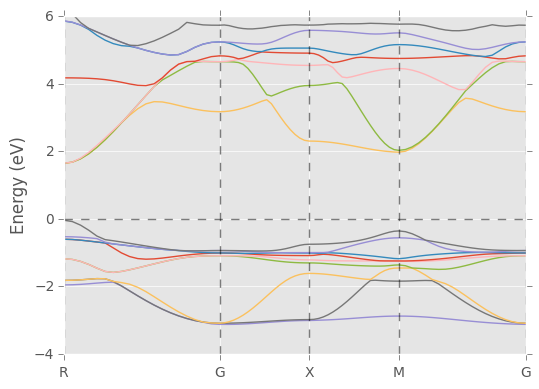
Returned dictionary:
{'data': {'columns': ['k_points',
              'band_1', 'band_2', 'band_3', 'band_4', 'band_5', 'band_6', 'band_7', 'band_8',
              'band_9', 'band_10', 'band_11', 'band_12', 'band_13', 'band_14', 'band_15', 'band_16',
              'band_17', 'band_18', 'band_19', 'band_20', 'band_21', 'band_22', 'band_23', 'band_24',
              'band_25', 'band_26', 'band_27', 'band_28', 'band_29', 'band_30', 'band_31', 'band_32'],
          'data': array(
            [[  0.        , -20.342219  , -16.616756  , ...,   5.849101  ,
                5.855091  ,   6.074841  ],
             [  0.04558028, -20.342181  , -16.616823  , ...,   5.811826  ,
                5.815311  ,   6.060851  ],
             [  0.09116057, -20.34223   , -16.617067  , ...,   5.730248  ,
                5.734556  ,   5.80481   ],
             ...,
             [  2.49869989, -20.343194  , -16.628521  , ...,   5.172637  ,
                5.204402  ,   5.711173  ],
             [  2.53591604, -20.343228  , -16.6286    , ...,   5.219897  ,
                5.226956  ,   5.730676  ],
             [  2.57313218, -20.34319   , -16.628622  , ...,   5.234177  ,
                5.234205  ,   5.726715  ]])},
 'reciprocal_point_locations': array([ 0.        ,  0.8660254 ,  1.3660254 ,  1.8660254 ,  2.57313218]),
 'reciprocal_points': ['R', 'G', 'X', 'M', 'G']}
Example: plotting total density of states with spin polarization
pydass_vasp.plotting.plot_tdos(axis_range=[-15, 15, 0, 40], return_refs=True)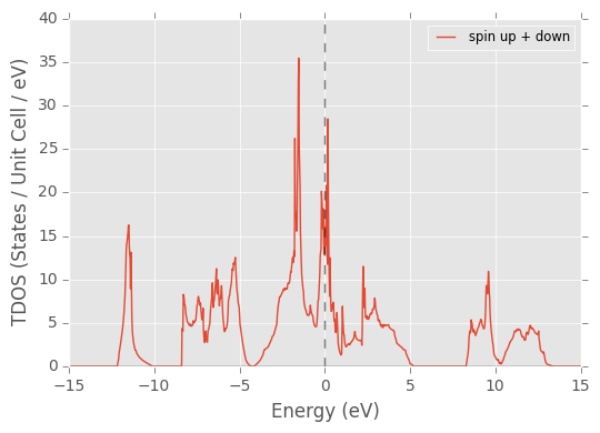
Returned dictionary:
{'ax_spin_combined': <matplotlib.axes._subplots.AxesSubplot at 0x108b95110>,
 'ax_spin_overlapping': <matplotlib.axes._subplots.AxesSubplot at 0x10b0f5fd0>,
 'data_spin_down': {'columns': ['E', 'total_down', 'integrated_down'],
  'data': array([[-22.63140452,   0.        ,   0.        ],
                 [-22.60640452,   0.        ,   0.        ],
                 [-22.58040452,   0.        ,   0.        ],
                 ...,
                 [ 15.05159548,   0.        ,  56.        ],
                 [ 15.07659548,   0.        ,  56.        ],
                 [ 15.10159548,   0.        ,  56.        ]])},
 'data_spin_up': {'columns': ['E', 'total_up', 'integrated_up'],
  'data': array([[-22.63140452,   0.        ,   0.        ],
                 [-22.60640452,   0.        ,   0.        ],
                 [-22.58040452,   0.        ,   0.        ],
                 ...,
                 [ 15.05159548,   0.        ,  56.        ],
                 [ 15.07659548,   0.        ,  56.        ],
                 [ 15.10159548,   0.        ,  56.        ]])}}
What is it?
This Python package is the result of frustration of searching for an organized, straightforward and flexible approach of plotting, fitting and manipulation of VASP files (typically POSCAR) in a few key strokes as long as you have a terminal, and preferably a (S)FTP client. It has the following features:
It is a Python package with a straightforward structure. When you import pydass_vasp, you have sub-packages pydass_vasp.plotting, pydass_vasp.fitting, pydass_vasp.manipulation, pydass_vasp.xml_utils, each containing a few functions to carry out your tasks, with a careful selection of options to choose from. Return values are Python dictionaries, informative enough to be flexible for post-processing. When there is no need for an object, don’t bother creating one.
It also has scripts that utilize the main package. They are simply ‘wrappers’ to the functions that are used the most frequently, typically plotting and fitting functions. Instead of cding into a directory and launching the Python interpreter python, making the imports and calling the functions, you just need to stay in your terminal shell and type plot_tdos.py to plot the total density of states (DOS), plot_ldos.py 1 to plot the local projected DOS of the first atom, and plot_bs.py to plot the band structure. These scripts accept arguments and options as flexible as their function counterparts.
The defaults of the functions and wrapping scripts are sane and cater to the most use cases. For example, If you are in a Python interpreter, simply typing in pydass_vasp.plotting.plot_tdos() will collect data to plot from DOSCAR and parameters necessary under the current VASP job directory, generate and display a figure (or more) but not save it/them on disk, and at the same time return a dictionary with the extracted data. It’ll automatically obtain critical parameters such as ISPIN, E-fermi first from VASP output files (e.g. OUTCAR), then input files (e.g. INCAR) if the first attempt fails, and decide the number of figures to generate. If you are just in a terminal shell, typing in the script plot_tdos.py will do the same, but rather than display the figure(s), instead, save it/them quietly and use matplotlib’s Agg backend. This would be particularly helpful for terminal users who don’t have X Window forwarding (Xming for Windows, XQuartz for Mac OS X) set up on their own local machine, or the forwarding connection is slow to hold the live generated figures.
The options to the functions and wrapping scripts provide you with room of customization from the beginning. For example, the internal documentation of pydass_vasp.plotting.plot_tdos() looks like below.
# see the docstring

# in IPython interpreter
pydass_vasp.plotting.plot_tdos?

# or in regular python interpreter
help(pydass_vasp.plotting.plot_tdos)
Plot the total density of states, with consideration of spin-polarization. Accepts input file 'DOSCAR', or 'vasprun.xml'. Parameters ---------- axis_range: list the range of axes x and y, 4 values in a list ISPIN: int user specified ISPIN If not given, for DOSCAR-type input, infer from OUTCAR/INCAR. For vasprun.xml-type input, infer from 'vasprun.xml'. input_file: string input file name, default to 'DOSCAR' For DOSCAR-type, can be any string containing 'DOSCAR'. For vasprun.xml-type input, can be any string ending with '.xml'. display: bool Display figures or not. Default to True. on_figs: list/int the current figure numbers to plot to, default to new figures return_refs: bool Return the axes reference(s) drawing or not. Default to False. save_figs: bool Save figures or not. Default to False. save_data: bool Save data or not. Default to False. output_prefix: string prefix string before the output files, default to 'TDOS' return_states_at_Ef: bool Calculate the TDOS at Ef with a 0.4 eV window of integration or not. Default to False. Returns ------- a dict, containing 'data': a dict that has 2D array of data, easily to Pandas DataFrame by pd.DataFrame(**returned_dict['data']) 'ax': the axes reference, if return_refs == TrueThe returned dictionary also leave room for adjustments. Take pydass_vasp.plotting.plot_tdos(return_refs=True) as an example.
returned_dict = {
    'data': {'columns': col_names, 'data': data}
    'ax': ax
}
returned_dict['data'] has a 2D numpy array of data, and their column names. This construction is prefered because if you have pandas, you can just convert it to a DataFrame by pd.DataFrame(**returned_dict['data']).
returned_dict['ax'] is the matplotlib axes reference. When ISPIN is 2, they are two elements: 'ax_spin_up' and 'ax_spin_down'.
It has a uniform plotting support for the Crystal Orbital Hamilton Populations (COHP) analysis tool LOBSTER, function pydass_vasp.plotting.plot_cohp() and script plot_cohp.py.
If you use matplotlib >= 1.4, and you plot with the wrapping scripts, you can optionally enjoy the aesthetic enhancement powered by its newly added sub-package style. For example, plot_tdos.py --style=ggplot switches on the style of ggplot. Read the stylesheet guide for more info, including designing and loading your own styles.
More on options
As an example, we again consider pydass_vasp.plotting.plot_tdos(), shortened as plot_tdos().
plot_tdos(input_file='vasprun.xml') switches from taking in DOSCAR to vasprun.xml. It lets you select what file you prefer to use. Any filename containing 'DOSCAR' is considered to be of DOSCAR type, any filename ending with '.xml' is considered to be of vasprun.xml type.
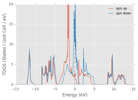
plot_tdos(ISPIN=2) lets you manually override the auto-detection of ISPIN from files other than DOSCAR. The program will skip the corresponding part of work. This is helpful when you only have the major data file DOSCAR transferred to you local machine, and do not have the other files necessary to extract the parameters to proceed plotting. To leave no confusion, when ISPIN is 2, two figures are generated, one with spin up and down combined, the other with two overlapping curves, denoting spin up and spin down separately.
plot_tdos(on_figs=1) creates the plot on top of an existing matplotlib figure labeled as Figure 1, instead of generating a whole new one.
plot_tdos(on_figs=[1,2]) when ISPIN is 2 puts the two plots mentioned before onto Figure 1 and Figure 2. plot_tdos(on_figs=[1,None]) is also valid, meaning putting the combined curve to Figure 1, and the two overlapping curves to a new figure, which you can of course delete on its own.
plot_tdos(display=False, save_figs=True) replicates the behavior of the corresponding wrapping script plot_tdos.py.
plot_tdos(return_refs=True) adds the matplotlib axes reference(s) to the returned dictionary, and keeps the figure(s) open to let you make further changes. Note: you don’t need to switch display on to get axes references.
plot_tdos(save_data=True, output_prefix='TDOS') saves the extracted data to disk, with the prefix 'TDOS'. The argument output_prefix also specifies the filenames for saved figures.
The wrapping script plot_tdos.py accepts the relevant options in the form of -i vasprun.xml, or --input vasprun.xml, -p or --display. For more readily available information, type in plot_tdos.py -h to get help direclty from the terminal shell.
Dependencies
Python 2.7 (Python 3 support is currently not considered)
NumPy
SciPy
matplotlib
IPython (optional, but better to have)
I highly recommend every scientist/researcher who is new to Python to install the scientific superpack Anaconda, if you are using Windows or Mac OS X. Even if you are on Linux, it is still highly recommended if you don’t have superuser control over the machine to install packages freely. It is often the case when you have ssh access to a supercomputer. In all these cases, just download the package and do a simple local installation, and you already have everything to start with, not only for pydass_vasp, but also for the whole adventure of scientific computing.
Installation
[STRIKEOUT:This package has already been registered on PyPI.] So if you have pip, which is a must have, and should already have been included in Anaconda,
[STRIKEOUT:pip install pydass_vasp]
[STRIKEOUT:Or] if you wish to follow the more updated releases, which should serve you better because small projects can fully enjoy the freedom of updates on GitHub before committing to PyPI,
pip install git+https://github.com/terencezl/pydass_vasp
Alternatively, if you don’t have pip, [STRIKEOUT:download the .tar.gz file from the PyPI page and decompress it in a local directory of your choice, or] git clone https://github.com/terencezl/pydass_vasp, get into the outer pydass_vasp directory and
python setup.py install

# then you can get out of that directory and just delete it
cd ..
rm -r pydass_vasp
However, pip installation is always recommended, because of the ease of uninstallation,
pip uninstall pydass_vasp
Getting Help
An organized tutorial/documentation has not been ready yet, but the docstrings of functions are fairly complete. If you use IPython, which is also a must have, and should already have been included in Anaconda,
import pydass_vasp

# in IPython interpreter
pydass_vasp.plotting.plot_tdos?

# or in regular python interpreter
help(pydass_vasp.plotting.plot_tdos)
You will get help. Experiment on a few options and you’ll be quickly on your way.
In addition, the help texts of scripts (option -h when you call them in the terminal shell) are available as well.


