Straightforward numerical integration of ODE systems from SymPy.

Project description


pyodesys provides a straightforward way of numerically integrating systems of ordinary differential equations (intial value problems). It unifies the interface of several libraries for performing the numerical integration as well as several libraries for symbolic representation. It also provides a convenience class for representing and integrating ODE systems defined by symbolic expressions, e.g. SymPy expressions. This allows the user to write concise code and rely on pyodesys to handle the subtle differences between libraries.
The numerical integration is perfomed using eiher:
Note that implicit steppers which require a user supplied callback for calculating the jacobian is provided automatically by pyodesys.
The symbolic representation is abstracted by using sym.
When performance is of outmost importance, e.g. in model fitting where results are needed for a large set of initial conditions and parameters, the user may transparently rely on compiled native code (pyodesys can generate optimal C++ code). The major benefit is that there is no need to manually rewrite the corresponing expressions in another programming language.
Documentation
Autogenerated API documentation for latest stable release is found here: https://bjodah.github.io/pyodesys/latest (and the development version for the current master branch is found here: http://hera.physchem.kth.se/~pyodesys/branches/master/html).
Installation
Simplest way to install pyodesys and its (optional) dependencies is to use the conda package manager:
$ conda install -c bjodah pyodesys pytest
$ python -m pytest --pyargs pyodesys
alternatively you may also use pip:
$ python -m pip install --user pyodesys[all]
see setup.py for optional requirements.
Examples
The classic van der Pol oscillator (see examples/van_der_pol.py)
>>> from pyodesys.symbolic import SymbolicSys
>>> def f(t, y, p):
...     return [y[1], -y[0] + p[0]*y[1]*(1 - y[0]**2)]
...
>>> odesys = SymbolicSys.from_callback(f, 2, 1)
>>> xout, yout, info = odesys.integrate(10, [1, 0], [1], integrator='odeint', nsteps=1000)
>>> _ = odesys.plot_result()
>>> import matplotlib.pyplot as plt; plt.show()  # doctest: +SKIP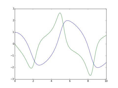
If the expression contains transcendental functions you will need to provide a backend keyword argument:
>>> import math
>>> from pyodesys.symbolic import SymbolicSys
>>> def f(x, y, p, backend=math):
...     return [backend.exp(-p[0]*y[0])]  # analytic: y(x) := ln(kx + kc)/k
...
>>> odesys = SymbolicSys.from_callback(f, 1, 1)
>>> y0, k = -1, 3
>>> xout, yout, info = odesys.integrate(5, [y0], [k], integrator='cvode', method='bdf')
>>> _ = odesys.plot_result()
>>> import matplotlib.pyplot as plt
>>> import numpy as np
>>> c = 1./k*math.exp(k*y0)  # integration constant
>>> _ = plt.plot(xout, np.log(k*(xout+c))/k, '--', linewidth=2, alpha=.5, label='analytic')
>>> _ = plt.legend(loc='best'); plt.show()  # doctest: +SKIP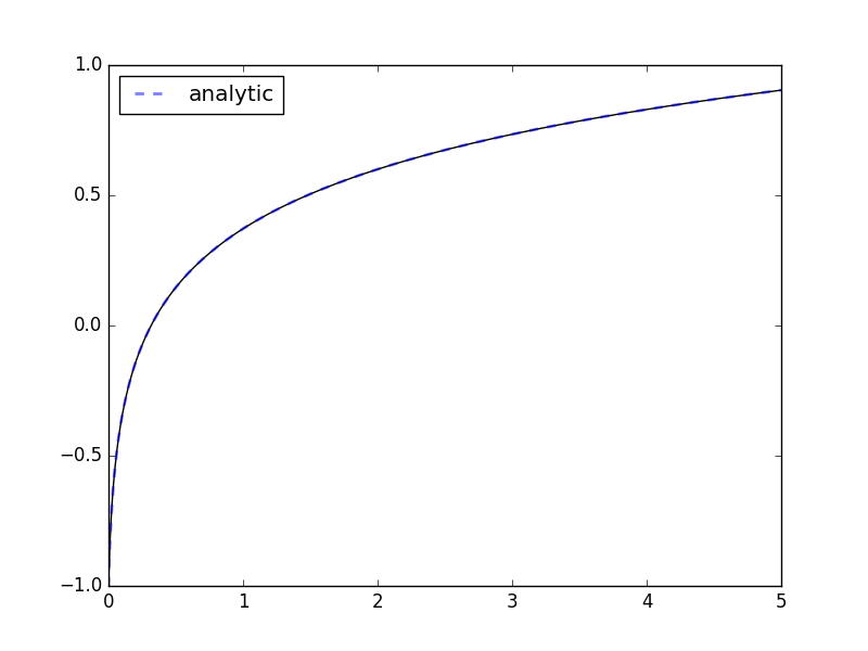
If you already have symbolic expressions created using e.g. SymPy you can create your system from those:
>>> import numpy as np
>>> import matplotlib.pyplot as plt
>>> import sympy as sp
>>> from pyodesys.symbolic import SymbolicSys
>>> t, u, v, k  = sp.symbols('t u v k')
>>> dudt = v
>>> dvdt = -k*u  # differential equations for a harmonic oscillator
>>> odesys = SymbolicSys([(u, dudt), (v, dvdt)], t, [k])
>>> result = odesys.integrate(7, {u: 2, v: 0}, {k: 3}, integrator='gsl', method='rk8pd', atol=1e-11, rtol=1e-12)
>>> _ = plt.subplot(1, 2, 1)
>>> _ = result.plot()
>>> _ = plt.subplot(1, 2, 2)
>>> _ = plt.plot(result.xout, 2*np.cos(result.xout*3**0.5) - result.yout[:, 0])
>>> plt.show()  # doctest: +SKIP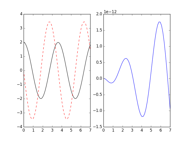
for more examples, see examples/, and rendered jupyter notebooks here: http://hera.physchem.kth.se/~pyodesys/branches/master/examples
License
The source code is Open Source and is released under the simplified 2-clause BSD license. See LICENSE for further details. Contributors are welcome to suggest improvements at https://github.com/bjodah/pyodesys
Release history Release notifications | RSS feed


Download files
Download the file for your platform. If you're not sure which to choose, learn more about installing packages.


