The ultimate anomaly detection library.

Project description
Anomalytics
Your Ultimate Anomaly Detection & Analytics Tool


Introduction
anomalytics is a Python library that aims to implement all statistical methods for the purpose of detecting any sort of anomaly e.g. extreme events, high or low anomalies, etc. This library utilises external dependencies such as:
- Pandas 2.1.1
- NumPy 1.26.0
- SciPy 1.11.3
- Matplotlib 3.8.2
- Pytest-Cov 4.1.0.
- Black 23.10.0
- Isort 5.12.0
- MyPy 1.6.1
- Bandit 1.7.5
anomalytics supports the following Python's versions: 3.10.x, 3.11.x, 3.12.0.
Installation
To use the library, you can install as follow:
# Install without openpyxl
$ pip3 install anomalytics

# Install with openpyxl
$ pip3 install "anomalytics[extra]"
As a contributor/collaborator, you may want to consider installing all external dependencies for development purposes:
# Install bandit, black, isort, mypy, openpyxl, pre-commit, and pytest-cov
$ pip3 install "anomalytics[codequality,docs,security,testcov,extra]"
Use Case
anomalytics can be used to analyze anomalies in your dataset (both as pandas.DataFrame or pandas.Series). To start, let's follow along with this minimum example where we want to detect extremely high anomalies in our dataset.
Read the walkthrough below, or the concrete examples here:
Anomaly Detection via the Detector Instance
-
Import
anomalyticsand initialise our time series of 100_002 rows:import anomalytics as atics df = atics.read_ts("./ad_impressions.csv", "csv") df.head()
               datetime	    xandr	      gam	    adobe
0	2023-10-18 09:01:00	52.483571	71.021131	35.681915
1	2023-10-18 09:02:00	49.308678	73.651996	60.347246
2	2023-10-18 09:03:00	53.238443	65.690813	48.120805
3	2023-10-18 09:04:00	57.615149	80.944393	59.550775
4	2023-10-18 09:05:00	48.829233	76.445099	26.710413
-
Initialize the needed detector object. Each detector utilises a different statistical method for detecting anomalies. In this example, we'll use POT method and a high anomaly type. Pay attention to the time period that is directly created where the
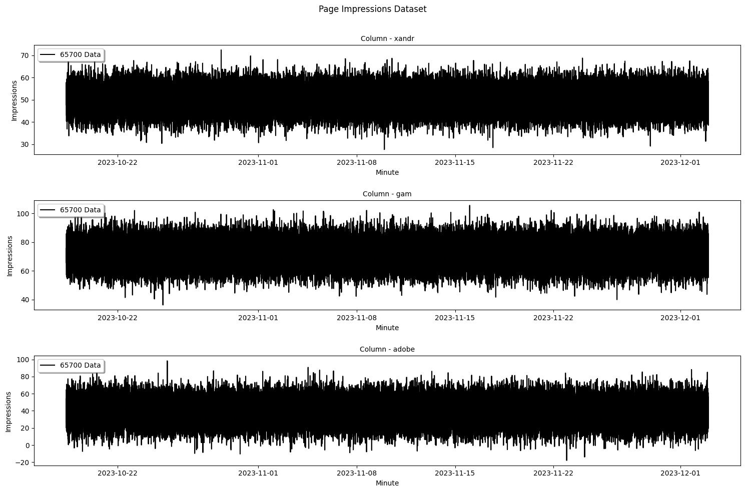
t2is 1 by default because "real-time" always targets the "now" period hence 1 (sec, min, hour, day, week, month, etc.):pot_detector = atics.get_detector(method="POT", dataset=ts, anomaly_type="high") print(f"T0: {pot_detector.t0}") print(f"T1: {pot_detector.t1}") print(f"T2: {pot_detector.t2}") pot_detector.plot(ptype="line-dataset-df", title=f"Page Impressions Dataset", xlabel="Minute", ylabel="Impressions", alpha=1.0)
T0: 42705
T1: 16425
T2: 6570
-
The purpose of using the detector object instead the standalone is to have a simple fix detection flow. In case you want to customize the time window, we can call the
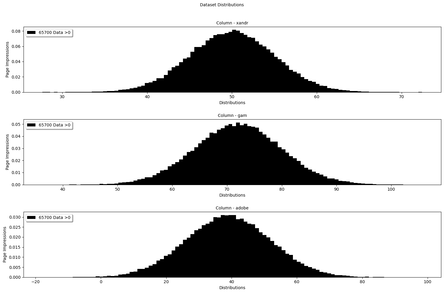
reset_time_window()to resett2value, even though that will beat the purpose of using a detector object. Pay attention to the period parameters because the method expects a percentage representation of the distribution of period (ranging 0.0 to 1.0):pot_detector.reset_time_window( "historical", t0_pct=0.65, t1_pct=0.25, t2_pct=0.1 ) print(f"T0: {pot_detector.t0}") print(f"T1: {pot_detector.t1}") print(f"T2: {pot_detector.t2}") pot_detector.plot(ptype="hist-dataset-df", title="Dataset Distributions", xlabel="Distributions", ylabel="Page Impressions", alpha=1.0, bins=100)
T0: 65001
T1: 25001
T2: 10000
-
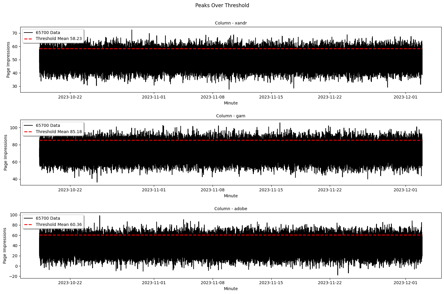
Now, we can extract exceedances by giving the expected
quantile:pot_detector.get_extremes(0.95) pot_detector.exeedance_thresholds.head()
        xandr	      gam	    adobe	           datetime
0	58.224653	85.177029	60.362306	2023-10-18 09:01:00
1	58.224653	85.177029	60.362306	2023-10-18 09:02:00
2	58.224653	85.177029	60.362306	2023-10-18 09:03:00
3	58.224653	85.177029	60.362306	2023-10-18 09:04:00
4	58.224653	85.177029	60.362306	2023-10-18 09:05:00
-
Let's visualize the exceedances and its threshold to have a clearer understanding of our dataset:
pot_detector.plot(ptype="line-exceedance-df", title="Peaks Over Threshold", xlabel="Minute", ylabel="Page Impressions", alpha=1.0)
-
Now that we have the exceedances, we can fit our data into the chosen distribution, in this example the "Generalized Pareto Distribution". The first couple rows will be zeroes which is normal because we only fit data that are greater than zero into the wanted distribution:
pot_detector.fit()
pot_detector.fit_result.head()
    xandr_anomaly_score gam_anomaly_score   adobe_anomaly_score	total_anomaly_score	           datetime
0	           1.087147	         0.000000              0.000000	           1.087147	2023-11-17 00:46:00
1	           0.000000	         0.000000              0.000000	           0.000000	2023-11-17 00:47:00
2	           0.000000	         0.000000              0.000000	           0.000000	2023-11-17 00:48:00
3	           0.000000	         1.815875              0.000000	           1.815875	2023-11-17 00:49:00
4	           0.000000	         0.000000              0.000000	           0.000000	2023-11-17 00:50:00
...
-
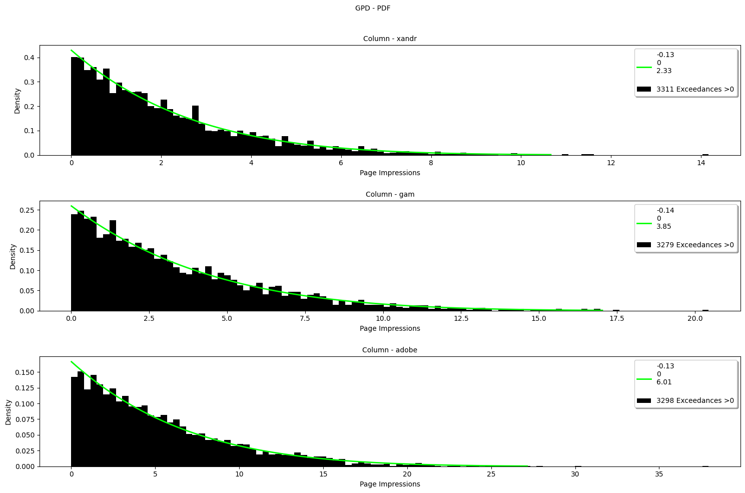
Let's inspect the GPD distributions to get the intuition of our pareto distribution:
pot_detector.plot(ptype="hist-gpd-df", title="GPD - PDF", xlabel="Page Impressions", ylabel="Density", alpha=1.0, bins=100)
-
The parameters are stored inside the detector class:
pot_detector.params
{0: {'xandr': {'c': -0.11675297447288158,
'loc': 0,
'scale': 2.3129766056305603,
'p_value': 0.9198385927065513,
'anomaly_score': 1.0871472537998},
'gam': {'c': 0.0,
'loc': 0.0,
'scale': 0.0,
'p_value': 0.0,
'anomaly_score': 0.0},
'adobe': {'c': 0.0,
'loc': 0.0,
'scale': 0.0,
'p_value': 0.0,
'anomaly_score': 0.0},
'total_anomaly_score': 1.0871472537998},
1: {'xandr': {'c': 0.0,
'loc': 0.0,
'scale': 0.0,
'p_value': 0.0,
'anomaly_score': 0.0},
'gam': {'c': 0.0,
'loc': 0.0,
'scale': 0.0,
'p_value': 0.0,
...
'scale': 0.0,
'p_value': 0.0,
'anomaly_score': 0.0},
'total_anomaly_score': 0.0},
...}
-
Last but not least, we can now detect the extremely large (high) anomalies:
pot_detector.detect(0.95)
pot_detector.detection_result
16425    False
16426    False
16427    False
16428    False
16429    False
        ...
22990    False
22991    False
22992    False
22993    False
22994    False
Name: detected data, Length: 6570, dtype: bool
-
Now we can visualize the anomaly scores from the fitting with the anomaly threshold to get the sense of the extremely large values:
pot_detector.plot(ptype="line-anomaly-score-df", title="Anomaly Score", xlabel="Minute", ylabel="Page Impressions", alpha=1.0)
-
Now what? Well, while the detection process seems quite straight forward, in most cases getting the details of each anomalous data is quite tidious! That's why
anomalyticsprovides a comfortable method to get the summary of the detection so we can see when, in which row, and how the actual anomalous data look like:pot_detector.detection_summary.head(5)
                          row	    xandr	      gam	    adobe	xandr_anomaly_score	gam_anomaly_score	adobe_anomaly_score	total_anomaly_score	anomaly_threshold
2023-11-28 12:06:00	    59225	64.117135	76.425925	47.772929	          21.445759	        0.000000	          0.000000	          21.445759	        19.689885
2023-11-28 12:25:00	    59244	40.513415	94.526021	65.921644	          0.000000	        19.557962	          2.685337	          22.243299	        19.689885
2023-11-28 12:45:00	    59264	52.362039	54.191719	79.972860	          0.000000	        0.000000	          72.313273	          72.313273	        19.689885
2023-11-28 16:48:00	    59507	64.753203	70.344142	42.540168	          32.543021	        0.000000	          0.000000	          32.543021	        19.689885
2023-11-28 16:53:00	    59512	35.912221	52.572939	75.621003	          0.000000	        0.000000	          22.199505	          22.199505	        19.689885
-
In every good analysis there is a test! We can evaluate our analysis result with "Kolmogorov Smirnov" 1 sample test to see how far the statistical distance between the observed sample distributions to the theoretical distributions via the fitting parameters (the smaller the
stats_distancethe better!):pot_detector.evaluate(method="ks") pot_detector.evaluation_result
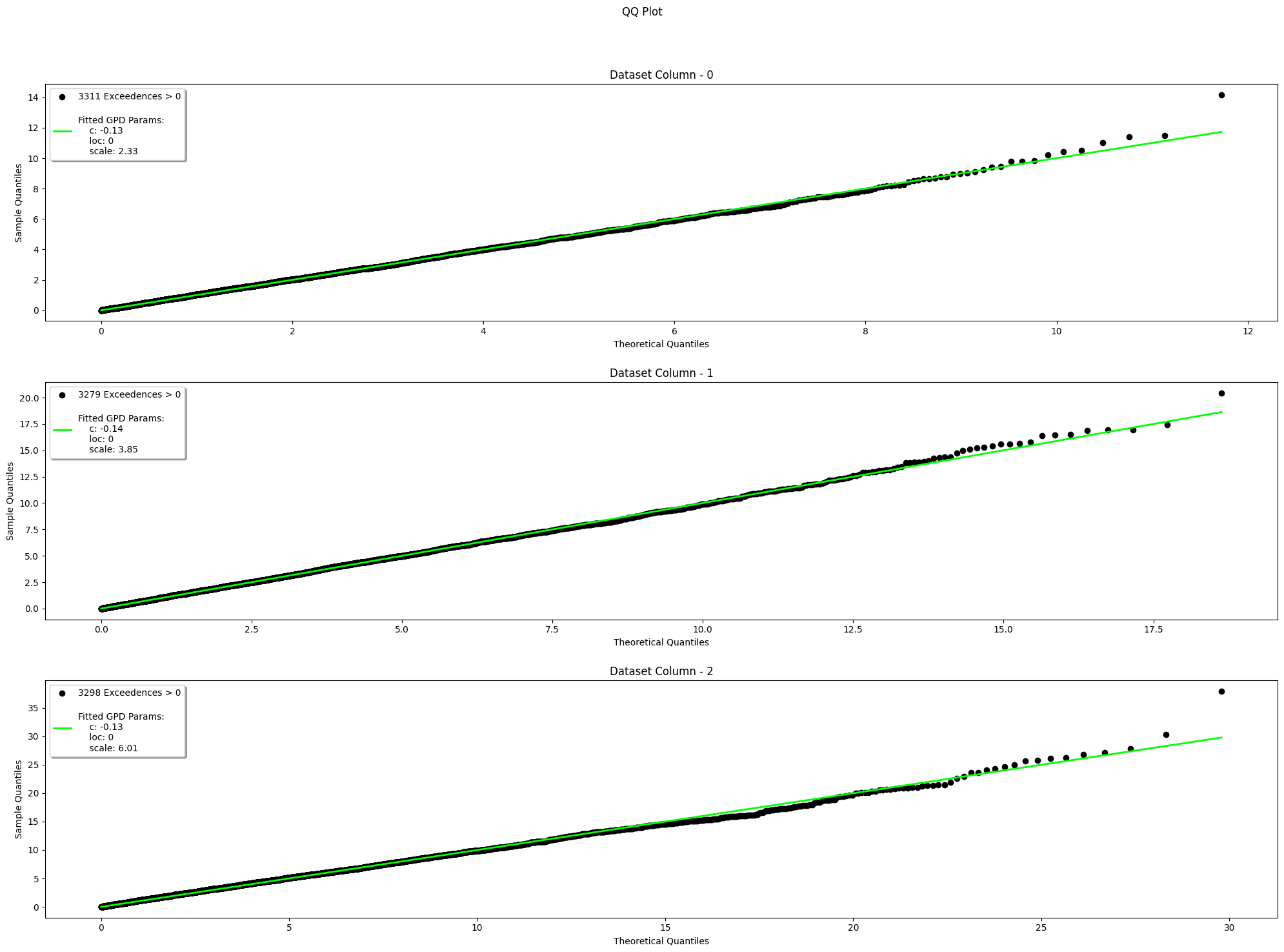
    column	total_nonzero_exceedances	stats_distance	p_value	        c	loc	    scale
0	 xandr	                     3311	      0.012901	0.635246 -0.128561	  0	 2.329005
1	 gam	                     3279	      0.011006	0.817674 -0.140479	  0	 3.852574
2	 adobe	                     3298	      0.019479	0.161510 -0.133019	  0	 6.007833
-
If 1 test is not enough for evaluation, we can also visually test our analysis result with "Quantile-Quantile Plot" method to observed the sample quantile vs. the theoretical quantile:
# Use the last non-zero parameters
pot_detector.evaluate(method="qq")

# Use a random non-zero parameters
pot_detector.evaluate(method="qq", is_random=True)

Anomaly Detection via Standalone Functions
You have a project that only needs to be fitted? To be detected? Don't worry! anomalytics also provides standalone functions as well in case users want to start the anomaly analysis from a different starting points. It is more flexible, but many processing needs to be done by you. LEt's take an example with a different dataset, thistime the water level Time Series!
-
Import
anomalyticsand initialise your time series:import anomalytics as atics ts = atics.read_ts( "water_level.csv", "csv" ) ts.head()
2008-11-03 06:00:00    0.219
2008-11-03 07:00:00   -0.041
2008-11-03 08:00:00   -0.282
2008-11-03 09:00:00   -0.368
2008-11-03 10:00:00   -0.400
Name: Water Level, dtype: float64
-
Set the time windows of t0, t1, and t2 to compute dynamic expanding period for calculating the threshold via quantile:
t0, t1, t2 = atics.set_time_window(
    total_rows=ts.shape[0],
    method="POT",
    analysis_type="historical",
    t0_pct=0.65,
    t1_pct=0.25,
    t2_pct=0.1
)

print(f"T0: {t0}")
print(f"T1: {t1}")
print(f"T2: {t2}")
T0: 65001
T1: 25001
T2: 10000
-
Extract exceedances and indicate that it is a
"high"anomaly type and what's thequantile:pot_thresholds = get_threshold_peaks_over_threshold(dataset=ts, t0=t0, "high", q=0.90) pot_exceedances = atics.get_exceedance_peaks_over_threshold( dataset=ts, threshold_dataset=pot_thresholds, anomaly_type="high" ) exceedances.head()
2008-11-03 06:00:00    0.859
2008-11-03 07:00:00    0.859
2008-11-03 08:00:00    0.859
2008-11-03 09:00:00    0.859
2008-11-03 10:00:00    0.859
Name: Water Level, dtype: float64
-
Compute the anomaly scores for each exceedance and initialize a params for further analysis and evaluation:
params = {}
anomaly_scores = atics.get_anomaly_score(
    exceedance_dataset=pot_exceedances,
    t0=t0,
    gpd_params=params
)

anomaly_scores.head()
2016-04-03 15:00:00    0.0
2016-04-03 16:00:00    0.0
2016-04-03 17:00:00    0.0
2016-04-03 18:00:00    0.0
2016-04-03 19:00:00    0.0
Name: anomaly scores, dtype: float64
...
-
Inspect the parameters:
params{0: {'index': Timestamp('2016-04-03 15:00:00'), 'c': 0.0, 'loc': 0.0, 'scale': 0.0, 'p_value': 0.0, 'anomaly_score': 0.0}, 1: {'index': Timestamp('2016-04-03 16:00:00'), ... 'c': 0.0, 'loc': 0.0, 'scale': 0.0, 'p_value': 0.0, 'anomaly_score': 0.0}, ...}
-
Detect anomalies:
anomaly_threshold = get_anomaly_threshold(
    anomaly_score_dataset=anomaly_scores,
    t1=t1,
    q=0.90
)
detection_result = get_anomaly(
    anomaly_score_dataset=anomaly_scores,
    threshold=anomaly_threshold,
    t1=t1
)

detection_result.head()
2020-03-31 19:00:00    False
2020-03-31 20:00:00    False
2020-03-31 21:00:00    False
2020-03-31 22:00:00    False
2020-03-31 23:00:00    False
Name: anomalies, dtype: bool
-
For the test, kolmogorov-smirnov and qq plot are also accessible via standalone functions, but the params need to be processed so it only contains a non-zero parameters since there are no reasons to calculate a zero 😂
nonzero_params = []

for row in range(0, t1 + t2):
    if (
        params[row]["c"] != 0
        or params[row]["loc"] != 0
        or params[row]["scale"] != 0
    ):
        nonzero_params.append(params[row])

ks_result = atics.evals.ks_1sample(
    dataset=pot_exceedances,
    stats_method="POT",
    fit_params=nonzero_params
)

ks_result
{'total_nonzero_exceedances': [5028], 'stats_distance': [0.0284] 'p_value': [0.8987], 'c': [0.003566], 'loc': [0], 'scale': [0.140657]}
-
Visualize via qq plot:
nonzero_exceedances = exceedances[exceedances.values > 0]

visualize_qq_plot(
    dataset=nonzero_exceedances,
    stats_method="POT",
    fit_params=nonzero_params,
)
Sending Anomaly Notification
We have anomaly you said? Don't worry, anomalytics has the implementation to send an alert via E-Mail or Slack. Just ensure that you have your email password or Slack webhook ready. This example shows both application (please read the comments 😎):
-
Initialize the wanted platform:
# Gmail
gmail = atics.get_notification(
    platform="email",
    sender_address="my-cool-email@gmail.com",
    password="AIUEA13",
    recipient_addresses=["my-recipient-1@gmail.com", "my-recipient-2@web.de"],
    smtp_host="smtp.gmail.com",
    smtp_port=876,
)

# Slack
slack = atics.get_notification(
    platform="slack",
    webhook_url="https://slack.com/my-slack/YOUR/SLACK/WEBHOOK",
)

print(gmail)
print(slack)
'Email Notification'
'Slack Notification'
-
Prepare the data for the notification! If you use standalone, you need to process the
detection_resultto become a DataFrame withrow, ``# Standalone detected_anomalies = detection_result[detection_result.values == True] anomalous_data = ts[detected_anomalies.index] standalone_detection_summary = pd.DataFrame( index=anomalous.index.flatten(), data=dict( row=[ts.index.get_loc(index) + 1 for index in anomalous.index], anomalous_data=[data for data in anomalous.values], anomaly_score=[score for score in anomaly_score[anomalous.index].values], anomaly_threshold=[anomaly_threshold] * anomalous.shape[0], ) ) # Detector Instance detector_detection_summary = pot_detector.detection_summary
-
Prepare the notification payload and a custome message if needed:
# Email
gmail.setup(
    detection_summary=detection_summary,
    message="Extremely large anomaly detected! From Ad Impressions Dataset!"
)

# Slack
slack.setup(
    detection_summary=detection_summary,
    message="Extremely large anomaly detected! From Ad Impressions Dataset!"
)
-
Send your notification! Beware that the scheduling is not implemented since it always depends on the logic of the use case:
# Email
gmail.send

# Slack
slack.send
'Notification sent successfully.' -
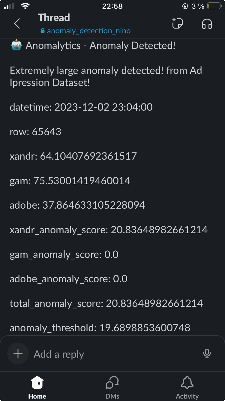
Check your email or slack, this example produces the following notification via Slack:
Reference
-
Nakamura, C. (2021, July 13). On Choice of Hyper-parameter in Extreme Value Theory Based on Machine Learning Techniques. arXiv:2107.06074 [cs.LG]. https://doi.org/10.48550/arXiv.2107.06074
-
Davis, N., Raina, G., & Jagannathan, K. (2019). LSTM-Based Anomaly Detection: Detection Rules from Extreme Value Theory. In Proceedings of the EPIA Conference on Artificial Intelligence 2019. https://doi.org/10.48550/arXiv.1909.06041
-
Arian, H., Poorvasei, H., Sharifi, A., & Zamani, S. (2020, November 13). The Uncertain Shape of Grey Swans: Extreme Value Theory with Uncertain Threshold. arXiv:2011.06693v1 [econ.GN]. https://doi.org/10.48550/arXiv.2011.06693
-
Yiannis Kalliantzis. (n.d.). Detect Outliers: Expert Outlier Detection and Insights. Retrieved [23-12-04T15:10:12.000Z], from https://detectoutliers.com/
Wall of Fame
I am deeply grateful to have met and guided by wonderful people who inspired me to finish my capstone project for my study at CODE university of applied sciences in Berlin (2023). Thank you so much for being you!
- Sabrina Lindenberg
- Adam Roe
- Alessandro Dolci
- Christian Leschinski
- Johanna Kokocinski
- Peter Krauß
Release history Release notifications | RSS feed


Download files
Download the file for your platform. If you're not sure which to choose, learn more about installing packages.
Source Distribution
Built Distribution
Hashes for anomalytics-0.2.2-py3-none-any.whl
| Algorithm | Hash digest | |
|---|---|---|
| SHA256 | ada5a1f5da7e55c6dfcd64e2c3a994504ed5c08827bf0f7ab25ef53e65b488f3 |
|
| MD5 | 9f24fec68bc2276eff681997333d4412 |
|
| BLAKE2b-256 | e4679bb9fbf852dee936c607dbabe1dce0b0fb958ed38aed799ea713e97d85b8 |


