Dynamic systems analysis

Project description
Caospy


Caospy is a Python package to analyze continuous dynamical systems and chaos.
Its utilities are:
- Solve systems of ODEs.
- Eigenvalues, eigenvectors and roots of equations.
- Classification of fixed points in 1D and 2D.
- Poincare maps.
- Plots.
Some well studied systems are available in the library, like Lorenz’s system, the Logistic equation, Duffing’s system and the Rosslers-Chaos systems.
Motivation
Dynamic sisytems are one of the most researched niches of knowledge, their understanding is crucial in order to interact more effectively with our environment. In order to study any dynamical systems to an acceptable level of detail, the classical qualitative analysis fall short and different heuristic methods along with numerical approaches where born to better understand their behavior. Properties like fixed points stability or chaotic behavior, and phenomena like bifurcations are commonly obtained by means of using these so called heuristic methods. Caospy attempts to bring this different tools of analysis together in one Python package, and achieve the unification and regularization of their use in a common developing context, hoping it will provide an easier and more comprehensive analysis of the subject in question.
Requirements
You will need Python 3.9 or later to run Caospy.
Installation
Caospy is available at PyPI. You can install it via the pip command:
$ pip install Caospy
If you'd like to bleeding edge of the code or you want to run the latest version, you can clone this repo and then inside the local directory execute:
$ pip install -e .
Usage
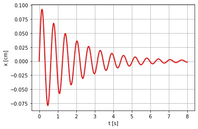
Let's study the damped harmonic oscillator without driving force. It's a second order one dimensional ODE, but we'll reduce it to a system of first-order odes.
import caospy as cp
import matplotlib.pyplot as plt


var = ["x", "y"] # Variables
par = ["k", "c"] # Parameters
fun = ["y", "-c*y-k*x"] # Functions
name = "Damped harmonic oscillator" # System's name
Ode_2d = cp.TwoDim(var, fun, par, name)

t0 = 0 # Initial time
tf = 8 # End time
x0 = [0, 1] # Initial Conditions
par_value = [100, 1] # Parameter values
N = 500 # Number of time steps
sol = Ode_2d.time_evolution(x0, par_value, t0, tf, N)

fig, ax = plt.subplots()
ax = sol.plot_trajectory("t-x") # Plot the solution
ax.set_xlabel("t [s]")
ax.set_ylabel("x [cm]")
You'll get the next figure.
For more examples, please refer to the tutorial in Documentation.
Contributing
Contributions are what make the open source community such an amazing place to learn, inspire, and create. Any contributions you make are greatly appreciated.
If you have a suggestion that would make this better, please fork the repo and create a pull request. You can also simply open an issue with the tag "enhancement". Don't forget to give the project a star! Thanks again!
- Fork the Project
- Create your Feature Branch (
git checkout -b feature/AmazingFeature) - Commit your Changes (
git commit -m 'Add some AmazingFeature') - Push to the Branch (
git push origin feature/AmazingFeature) - Open a Pull Request
License
Distributed under the MIT License. See LICENSE for more information.
Authors
Juan Colman(E-mail: juancolmanot@gmail.com), Sebastián Nicolás Bertolo.
Release history Release notifications | RSS feed

Download files
Download the file for your platform. If you're not sure which to choose, learn more about installing packages.


