evident

Evident is a tool for performing effect size and power calculations on microbiome diversity data.

Installation

You can install the most up-to-date version of evident from PyPi using the following command:

pip install evident

QIIME 2

evident is also available as a QIIME 2 plugin. Make sure you have activated a QIIME 2 environment and run the same installation command as above.

To check that evident installed correctly, run the following from the command line:

qiime evident --help

You should see something like this if evident installed correctly:

Usage: qiime evident [OPTIONS] COMMAND [ARGS]...

  Description: Perform power analysis on microbiome diversity data. Supports
  calculation of effect size given metadata covariates and supporting
  visualizations.

  Plugin website: https://github.com/gibsramen/evident

  Getting user support: Please post to the QIIME 2 forum for help with this
  plugin: https://forum.qiime2.org

Options:
  --version            Show the version and exit.
  --example-data PATH  Write example data and exit.
  --citations          Show citations and exit.
  --help               Show this message and exit.

Commands:
  alpha-effect-size-by-category  Alpha diversity effect size by category.
  alpha-power-analysis           Alpha diversity power analysis.
  beta-effect-size-by-category   Beta diversity effect size by category.
  beta-power-analysis            Beta diversity power analysis.
  plot-power-curve               Plot power curve.
  visualize-results              Tabulate evident results.

Usage

evident requires two input files:

1. Either an alpha or beta diversity file
2. Sample metadata

First, open Python and import evident

import evident

Next, load your diversity file and sample metadata. For alpha diversity, this should be a pandas Series. For beta diversity, this should be an scikit-bio DistanceMatrix. Sample metadata should be a pandas DataFrame. We'll be using an alpha diversity vector for this tutorial but the commands are nearly the same for beta diversity distance matrices.

import pandas as pd

metadata = pd.read_table("data/metadata.tsv", sep="\t", index_col=0)
faith_pd = metadata["faith_pd"]

The main data structure in evident is the 'DiversityHandler'. This is the way that evident stores the diversity data and metadata for power calculations. For our alpha diversity example, we'll load the AlphaDiversityHandler class from evident. AlphaDiversityHandler takes as input the pandas Series with the diversity values and the pandas DataFrame containing the sample metadata.

adh = evident.AlphaDiversityHandler(faith_pd, metadata)

Next, let's say we want to get the effect size of the diversity differences between two groups of samples. We have in our example a column in the metadata "classification" comparing two groups of patients with Crohn's disease. First, we'll look at the mean of Faith's PD between these two groups.

metadata.groupby("classification").agg(["count", "mean", "std"])["faith_pd"]

which results in

                count       mean       std
classification
B1                 99  13.566110  3.455625
Non-B1            121   9.758946  3.874911

Looks like there's a pretty large difference between these two groups. What we would like to do now is calculate the effect size of this difference. Because we are comparing only two groups, we can use Cohen's d. evident automatically chooses the correct effect size to calculate - either Cohen's d if there are only two categories or Cohen's f if there are more than 2.

adh.calculate_effect_size(column="classification")

This tells us that our effect size is 1.03.

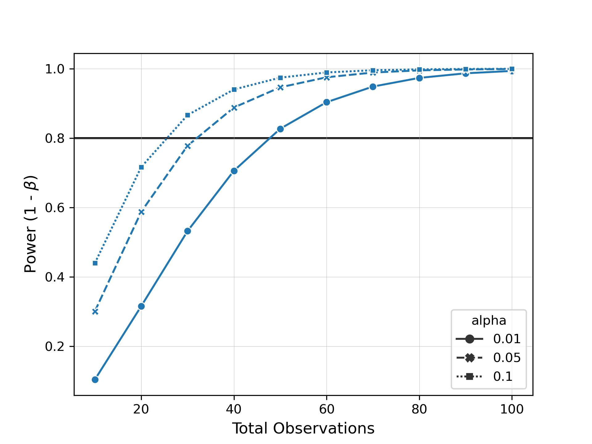
Now let's say we want to see how many samples we need to be able to detect this difference with a power of 0.8. evident allows you to easily specify arguments for alpha, power, or total observations for power analysis. We can then plot these results as a power curve to summarize the data.

from evident.plotting import plot_power_curve
import numpy as np

alpha_vals = [0.01, 0.05, 0.1]
obs_vals = np.arange(10, 101, step=10)
results = adh.power_analysis(
    "classification",
    alpha=alpha_vals,
    total_observations=obs_vals
)
plot_power_curve(results, target_power=0.8, style="alpha", markers=True)

When we inspect this plot, we can see how many samples we would need to collect to observe the same effect size at different levels of significance and power.