Quantitative, Fast Grid-Based Fields Calculations in 2D and 3D - Residence Time Distributions, Velocity Grids, Eulerian Cell Projections etc.

Project description


Quantitative, Fast Grid-Based Fields Calculations in 2D and 3D - Residence Time Distributions, Velocity Grids, Eulerian Cell Projections etc.
That sounds dry as heck.
Project moving particles' trajectories (experimental or simulated) onto 2D or 3D grids with infinite resolution.
Better? No? Here are some figures produced by KonigCell:
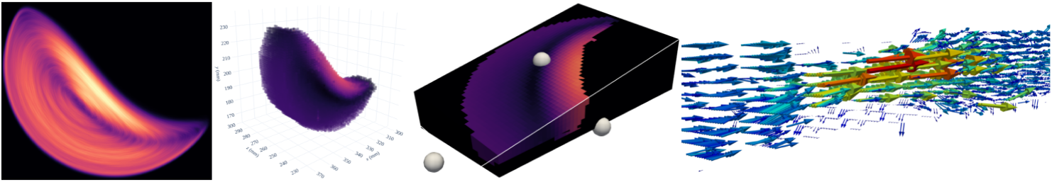
Left panel: 2D residence time distribution in a GranuTools GranuDrum imaged using Positron Emission Particle Tracking (PEPT). Two middle panels: 3D velocity distribution in the same system; voxels are rendered as a scatter plot (left) and tomogram-like 3-slice (right). Right panel: velocity vectorfield in a constricted pipe simulating a aneurysm, imaged using PEPT.
This is, to my knowledge, the only library that accurately projects particle trajectories onto grids - that is, taking their full projected area / volume into account (and not approximating them as points / lines). It's also the only one creating quantitative 3D projections.
And it is fast - 1,000,000 particle positions can be rasterized onto a 512x512 grid in 7 seconds on my 16-thread i9 CPU. The code is fully parallelised on threads, processes or distributed MPI nodes.
But Why?
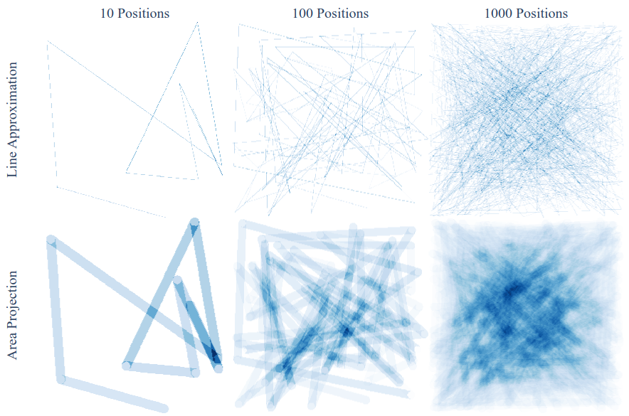
Rasterizing moving tracers onto uniform grids is a powerful way of computing statistics about a system - occupancies, velocity vector fields, modelling particle clump imaging etc. - be it experimental or simulated. However, the classical approach of approximating particle trajectories as lines discards a lot of (most) information.
Here is an example of a particle moving randomly inside a box - on a high resolution (512x512) pixel grid, the classical approach (top row) does not yield much better statistics with increasing numbers of particle positions imaged. Projecting complete trajectory areas onto the grid (KonigCell, bottom row) preserves more information about the system explored:
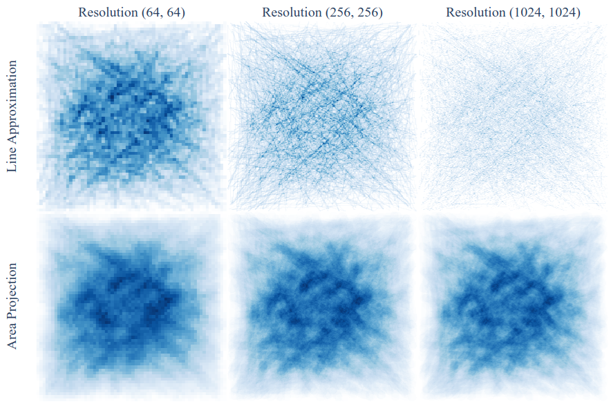
A typical strategy for dealing with information loss is to coarsen the pixel grid, resulting in a trade-off between accuracy and statistical soundness. However, even very low resolutions still yield less information using line approximations (top row). With area projections, you can increase the resolution arbitrarily and improve precision (KonigCell, bottom row):
The KonigCell Libraries
This repository effectively hosts three libraries:
konigcell2d: a portable C library for 2D grid projections.konigcell3d: a portable C library for 3D grid projections.konigcell: a user-friendly Python interface to the two libraries above.
Installing the Python Package
This package supports Python 3.6 and above (though it might work with even older versions).
Install this package from PyPI:
pip install konigcell
Or conda-forge:
conda install konigcell
If you have a relatively standard system, the above should just download pre-compiled wheels - so no prior configuration should be needed.
To build this package on your specific machine, you will need a C compiler - the low-level C code does not use any tomfoolery, so any compiler since the 2000s should do.
To build the latest development version from GitHub:
pip install git+https://github.com/anicusan/KonigCell
Integrating the C Libraries with your Code
The C libraries in the konigcell2d and konigcell3d directories in this repository; they
contain instructions for compiling and using the low-level subroutines. All code is fully
commented and follows a portable subset of the C99 standard - so no VLAs, weird macros or
compiler-specific extensions. Even MSVC compiles it!
You can run make in the konigcell2d or konigcell3d directories to build shared
libraries and the example executables under -Wall -Werror -Wextra like a stickler. Running
make in the repository root builds both libraries.
Both libraries are effectively single-source - they should be as straightforward as possible to integrate in other C / C++ codebases, or interface with from higher-level programming languages.
Examples and Documentation
The examples directory contains some Python scripts using the high-level Python routines
and the low-level Cython interfaces. The konigcell2d and konigcell3d directories contain
C examples.
Full documentation is available here.
import numpy as np
import konigcell as kc
# Generate a short trajectory of XY positions to pixellise
positions = np.array([
[0.3, 0.2],
[0.2, 0.8],
[0.3, 0.55],
[0.6, 0.8],
[0.3, 0.45],
[0.6, 0.2],
])
# The particle radius may change
radii = np.array([0.05, 0.03, 0.01, 0.02, 0.02, 0.03])
# Values to rasterize - velocity, duration, etc.
values = np.array([1, 2, 1, 1, 2, 1])
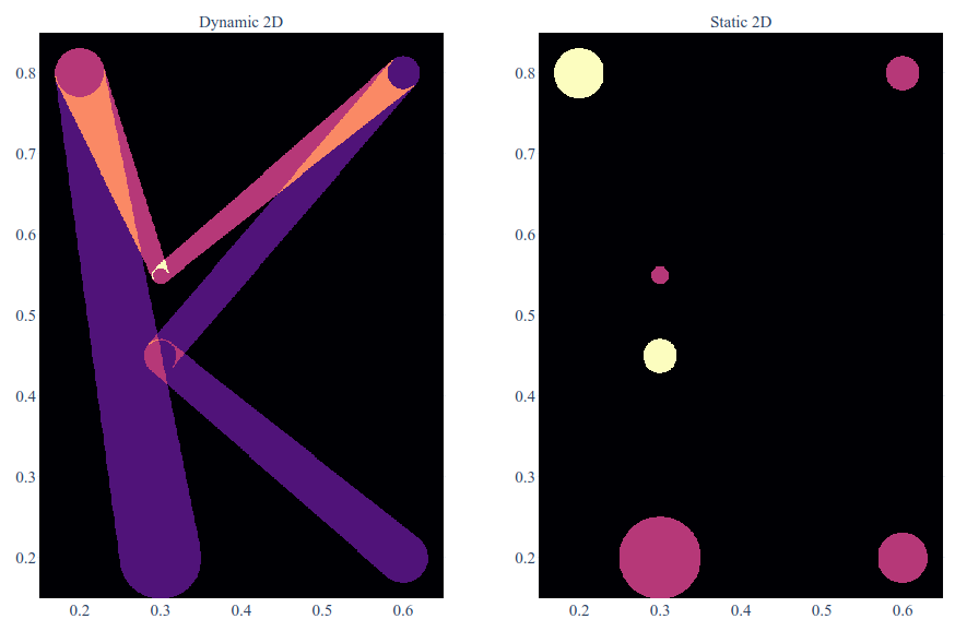
# Pixellise the particle trajectories
pixels1 = kc.dynamic2d(
positions,
mode = kc.ONE,
radii = radii,
values = values[:-1],
resolution = (512, 512),
)
pixels2 = kc.static2d(
positions,
mode = kc.ONE,
radii = radii,
values = values,
resolution = (512, 512),
)
# Create Plotly 1x2 subplot grid and add Plotly heatmaps of pixels
fig = kc.create_fig(
nrows = 1, ncols = 2,
subplot_titles = ["Dynamic 2D", "Static 2D"],
)
fig.add_trace(pixels1.heatmap_trace(), row = 1, col = 1)
fig.add_trace(pixels2.heatmap_trace(), row = 1, col = 2)
fig.show()
Contributing
You are more than welcome to contribute to this library in the form of library improvements, documentation or helpful examples; please submit them either as:
- GitHub issues.
- Pull requests (superheroes only).
- Email me at a.l.nicusan@bham.ac.uk.
Acknowledgements
I would like to thank the Formulation Engineering CDT @School of Chemical Engineering and the Positron Imaging Centre @School of Physics and Astronomy, University of Birmingham for supporting my work.
And thanks to Dr. Kit Windows-Yule for putting up with my bonkers ideas.
Citing
If you use this library in your research, you are kindly asked to cite:
[Paper after publication]
This library would not have been possible without the excellent r3d library
(https://github.com/devonmpowell/r3d) which forms the very core of the C
subroutines; if you use KonigCell in your work, please also cite:
Powell D, Abel T. An exact general remeshing scheme applied to physically conservative voxelization. Journal of Computational Physics. 2015 Sep 15;297:340-56.
Licensing
KonigCell is MIT licensed. Enjoy.


Download files
Download the file for your platform. If you're not sure which to choose, learn more about installing packages.
Source Distribution
Built Distributions
Hashes for konigcell-0.2.1-cp310-cp310-win_amd64.whl
| Algorithm | Hash digest | |
|---|---|---|
| SHA256 | cff78b65375c9dabd49cd0dfefda752da0ef0fcec29c4f9d7d5313e3da5b7fcd |
|
| MD5 | be7c3afd5154d217c0f1819b4bc8f43d |
|
| BLAKE2b-256 | 4ee1e0561aa71431bf64a15100c4596621b815994df30062c4dd56af9e00eaad |
Hashes for konigcell-0.2.1-cp310-cp310-win32.whl
| Algorithm | Hash digest | |
|---|---|---|
| SHA256 | 642e1f23342448fc291199df4459db3c99442b3d9b02e1f9da5d3d18e1cbf022 |
|
| MD5 | 0ec226968ec193470a0bec2dc703f6da |
|
| BLAKE2b-256 | 64ef7a27fed7e1232c15b731ba150255674b13701bb06e1fe173be49e0073582 |
Hashes for konigcell-0.2.1-cp310-cp310-manylinux_2_5_x86_64.manylinux1_x86_64.manylinux_2_12_x86_64.manylinux2010_x86_64.whl
| Algorithm | Hash digest | |
|---|---|---|
| SHA256 | 5b3a97026a8901fe26bac285537c482391afd306eef4bc6f8fe6e9cba86ca452 |
|
| MD5 | 4c1166455a61675ca0a05d8b6615f0aa |
|
| BLAKE2b-256 | 72f2479ca6e52827d7a26c3b13cdd727b33c1e396e9a2bee9ee26b442e5bbf9b |
Hashes for konigcell-0.2.1-cp310-cp310-manylinux_2_5_i686.manylinux1_i686.manylinux_2_12_i686.manylinux2010_i686.whl
| Algorithm | Hash digest | |
|---|---|---|
| SHA256 | 758f5bdbe4a6e143203e605cbe18c872e96d62744a4a660d87d2e64909b16be3 |
|
| MD5 | c23bfd71ca89abcb1ec29032a05290e9 |
|
| BLAKE2b-256 | d8935eacb2f6db2b3ef659646d2df401b8b14cb65b0a41c4428f974800af6898 |
Hashes for konigcell-0.2.1-cp310-cp310-macosx_10_9_x86_64.whl
| Algorithm | Hash digest | |
|---|---|---|
| SHA256 | 93bdbb6b7fb3fbdf4ecdbd7504698c43bf2b3f39aa5952a4dad5c046e74ea466 |
|
| MD5 | 2d40b5a697f3c7dba96dd8cea54766cf |
|
| BLAKE2b-256 | 0d4c0e826cd20ed46712178c655004ee57cd3e2a3f6466ed7a2a23ec6b93c01e |
Hashes for konigcell-0.2.1-cp39-cp39-win_amd64.whl
| Algorithm | Hash digest | |
|---|---|---|
| SHA256 | e545b7899d4f20dec2997630a9b524193c63d441fcc0da716062db80caee870d |
|
| MD5 | 0cccff25fae9aed303280b44a148608d |
|
| BLAKE2b-256 | 6294855a49efa1b2ad863f500eed0978aecbbe61231784f0289bcebd301ef052 |
Hashes for konigcell-0.2.1-cp39-cp39-win32.whl
| Algorithm | Hash digest | |
|---|---|---|
| SHA256 | 235295bea38a6911a113bad7af53884c4bf52946980bfd0fe54a143d1e338948 |
|
| MD5 | e3fd690ed5b41f7a54f8464d81f1805a |
|
| BLAKE2b-256 | c6f561fc1d8f5009133895f40a314a540246d902040e7baf5c6a96861384cfe5 |
Hashes for konigcell-0.2.1-cp39-cp39-manylinux_2_5_x86_64.manylinux1_x86_64.manylinux_2_12_x86_64.manylinux2010_x86_64.whl
| Algorithm | Hash digest | |
|---|---|---|
| SHA256 | fa8029e1bade31eea7f7aaf6367bab52491133582e69abdce67dd6e66e7c148c |
|
| MD5 | b67096d25a2aa02cdbd71ef5dd7b6991 |
|
| BLAKE2b-256 | d43588a986b983e146b5718ad44f9e16737762826c0b8cff5852545c318eff57 |
Hashes for konigcell-0.2.1-cp39-cp39-manylinux_2_5_i686.manylinux1_i686.manylinux_2_12_i686.manylinux2010_i686.whl
| Algorithm | Hash digest | |
|---|---|---|
| SHA256 | d88747a325373e504712a537c4a709df0f980c837f34815e9bcb572d71a122c5 |
|
| MD5 | 6f50bda2af356bdc278b9565fc2541a0 |
|
| BLAKE2b-256 | 52ea47c7a2ead68708f670bbcf490e3d4e7703fe14fb249153830dcc38c51256 |
Hashes for konigcell-0.2.1-cp39-cp39-macosx_10_9_x86_64.whl
| Algorithm | Hash digest | |
|---|---|---|
| SHA256 | 9d9b5d8aa093da77fd7f16ceb73cfa78177b7a46f7dba63aada85d6192d627de |
|
| MD5 | ea8a39e60cc4106883f6fe148514d790 |
|
| BLAKE2b-256 | 45010edb1262c4a78171e8a81c2193d2a858461ee9b88c570acbc744615e2175 |
Hashes for konigcell-0.2.1-cp38-cp38-win_amd64.whl
| Algorithm | Hash digest | |
|---|---|---|
| SHA256 | 4dfe5f7abeaf157f008872045b6c01fca140f1aaf7b5e1d3849a12adfba201cc |
|
| MD5 | df29948f35f1e94c15fabd5be7badf2d |
|
| BLAKE2b-256 | beed49767132f8973f47cc79e9ae0daef50fcc2b21535e339427f4e8476aa073 |
Hashes for konigcell-0.2.1-cp38-cp38-win32.whl
| Algorithm | Hash digest | |
|---|---|---|
| SHA256 | c78597d4b2fbf31ff0d818835186875cb6844308c9e5dfaa1e39ba955573ce3f |
|
| MD5 | 9855ccd87bff7360b61027ee55b1afdd |
|
| BLAKE2b-256 | dfd91f8d538f915338e84c98014833f029e4a5ba7c222e1471b3ea116f0030c5 |
Hashes for konigcell-0.2.1-cp38-cp38-manylinux_2_5_x86_64.manylinux1_x86_64.manylinux_2_12_x86_64.manylinux2010_x86_64.whl
| Algorithm | Hash digest | |
|---|---|---|
| SHA256 | c928d37713e04b518ead24c51d681c764ae2b5752ca5140e9cc57d1700a771c6 |
|
| MD5 | cf8cac7772be98521ec8c1e2cf4bf386 |
|
| BLAKE2b-256 | 19fe9064d500314e0fff864ddc0f4263a8ed2b1cd8219f2c22491f3a884b7821 |
Hashes for konigcell-0.2.1-cp38-cp38-manylinux_2_5_i686.manylinux1_i686.manylinux_2_12_i686.manylinux2010_i686.whl
| Algorithm | Hash digest | |
|---|---|---|
| SHA256 | ef0f0e2447ae57b054bae48abd9b4d54e9257c662f8781d7cb4935f0e2c8f703 |
|
| MD5 | c7f3adebf422719b66853ae0fa8922db |
|
| BLAKE2b-256 | a0293213dd2c8c49806ffa1fdb8fda88dedc320a735186eb7801c9cc67e1e4ae |
Hashes for konigcell-0.2.1-cp38-cp38-macosx_10_9_x86_64.whl
| Algorithm | Hash digest | |
|---|---|---|
| SHA256 | 0188feb5db9f079d90406180bc9a638a0cd19cb031a70c68a033d4047c0e481b |
|
| MD5 | cf82b923dfab9c335e61892c5f22b3c1 |
|
| BLAKE2b-256 | addd7d6a1483be1743050ac4eb3c1ff933b7b6c739d5bc97bab1cc788186ce9f |
Hashes for konigcell-0.2.1-cp37-cp37m-win_amd64.whl
| Algorithm | Hash digest | |
|---|---|---|
| SHA256 | 118dd7a670173d912f54825bbd755613e2c887177fb6680c2a6ee3328002b754 |
|
| MD5 | a4da02b8f0da84d89417a60579b3dc90 |
|
| BLAKE2b-256 | 7a1e82757ae6f63327fc1aa50806641e7603afc7bbf970a25cebd64867e86d80 |
Hashes for konigcell-0.2.1-cp37-cp37m-win32.whl
| Algorithm | Hash digest | |
|---|---|---|
| SHA256 | c7dae26f807e6f9ffecdf559c6739b5da0866621816dc9fc8330b50a4369016c |
|
| MD5 | 78bf7125533c530bc4f06deac7947a31 |
|
| BLAKE2b-256 | 24967b4f48aff71f3e862e55358a5863ff82a36d96347e52b4be1f6f81120b94 |
Hashes for konigcell-0.2.1-cp37-cp37m-manylinux_2_5_x86_64.manylinux1_x86_64.manylinux_2_12_x86_64.manylinux2010_x86_64.whl
| Algorithm | Hash digest | |
|---|---|---|
| SHA256 | d52c95cf9ef3a77e476a05ab183d26c81a1349a2b41e1ba439d746009b4f3217 |
|
| MD5 | cef9d596f133e38a40cc3f65f57108ab |
|
| BLAKE2b-256 | c0e0a8770c3ca4d69a86d658a8c704adf18259b9673e08c27e1a34778b52e101 |
Hashes for konigcell-0.2.1-cp37-cp37m-manylinux_2_5_i686.manylinux1_i686.manylinux_2_12_i686.manylinux2010_i686.whl
| Algorithm | Hash digest | |
|---|---|---|
| SHA256 | fa2696cc61c49eba93e51b44554c43a7e8e4ef485ae00676437f86fce94e9a8b |
|
| MD5 | 540c1503d9e93bc910188515f4b37ddb |
|
| BLAKE2b-256 | 7daec665e8ae2f2674b533ba0c0112e62ed54090852e1add9249077f616ef861 |
Hashes for konigcell-0.2.1-cp37-cp37m-macosx_10_9_x86_64.whl
| Algorithm | Hash digest | |
|---|---|---|
| SHA256 | b59001e39b73fa7dac619c1750d33e3160b59d0539c70fb625b3e117c6f26e2f |
|
| MD5 | 0a214f7209a0d12f1447f070090b2fa9 |
|
| BLAKE2b-256 | 9281604f0b2bbc309ff7e162fb80a33ca6695db1f78edcef763f7955612c83ec |
Hashes for konigcell-0.2.1-cp36-cp36m-win_amd64.whl
| Algorithm | Hash digest | |
|---|---|---|
| SHA256 | b59ddb87e1ac980a37817371f23097caff967f3782f9356f3309f76ef3fe482c |
|
| MD5 | 90fedc6ebb7fdd7bdf1e64116afd3db5 |
|
| BLAKE2b-256 | c54a0695383f7972f4ea70101d0cc814e7ce32e70ddc98e3ba19322af7b29239 |
Hashes for konigcell-0.2.1-cp36-cp36m-win32.whl
| Algorithm | Hash digest | |
|---|---|---|
| SHA256 | c9e7e7960811ad5c4d73e4e83bf53ef55ddb3cfb639373181373557407fd6e59 |
|
| MD5 | a5a669eedbebab1951cd6945e20d7101 |
|
| BLAKE2b-256 | 38643580780097feca02b367ddbb2bb3517b9dcaad72c6c8c9e4be50fa2b5274 |
Hashes for konigcell-0.2.1-cp36-cp36m-manylinux_2_5_x86_64.manylinux1_x86_64.manylinux_2_12_x86_64.manylinux2010_x86_64.whl
| Algorithm | Hash digest | |
|---|---|---|
| SHA256 | 75b03fb57da697196243db020d144a8428cb2aea6e8912e49a5afdc5ae0e93cc |
|
| MD5 | f5f22c57081f6edf97b75f2d11dd0b19 |
|
| BLAKE2b-256 | 75339e2322c12dc9f5f05c9b3952967d338177fa20f036e315956951b7af36c3 |
Hashes for konigcell-0.2.1-cp36-cp36m-manylinux_2_5_i686.manylinux1_i686.manylinux_2_12_i686.manylinux2010_i686.whl
| Algorithm | Hash digest | |
|---|---|---|
| SHA256 | 0482b42affaf32a48d4de0cb3b22cf1b6b9c06b708028d1f893dc53c62284cfb |
|
| MD5 | bfc4595499abd66eb5a0708fe95a54c9 |
|
| BLAKE2b-256 | 9e478380db698cd600e26772532c3e9dcba0b9a208006ef3677fee6c1a81b285 |
Hashes for konigcell-0.2.1-cp36-cp36m-macosx_10_9_x86_64.whl
| Algorithm | Hash digest | |
|---|---|---|
| SHA256 | 3745dc2ca9fe706c1f16986a3173e71160d3534d6faac100ea2729fff5dd09b8 |
|
| MD5 | a9be051d03bc03bad0bd7f835c7a631c |
|
| BLAKE2b-256 | c2449ebc8669d3c867270c399514c9ba4a019f8eb4f2e326959fece647a90199 |


