Find the best probability distribution for your dataset

Project description


Phitter analyzes datasets and determines the best analytical probability distributions that represent them. Phitter studies over 80 probability distributions, both continuous and discrete, 3 goodness-of-fit tests, and interactive visualizations. For each selected probability distribution, a standard modeling guide is provided along with spreadsheets that detail the methodology for using the chosen distribution in data science, operations research, and artificial intelligence.
This repository contains the implementation of the python library and the kernel of Phitter Web
Installation
Requirements
python: >=3.9
PyPI
pip install phitter
Usage
Notebook's Tutorials
| Tutorial | Notebooks |
|---|---|
| Fit Continuous |  |
| Fit Discrete | |
| Fit Accelerate [Sample>100K] | |
| Fit Specific Disribution | |
| Working Distribution | |
General
import phitter

data: list[int | float] = [...]

phitter_cont = phitter.PHITTER(data)
phitter_cont.fit()
Full continuous implementation
import phitter

data: list[int | float] = [...]

phitter_cont = phitter.PHITTER(
    data=data,
    fit_type="continuous",
    num_bins=15,
    confidence_level=0.95,
    minimum_sse=1e-2,
    distributions_to_fit=["beta", "normal", "fatigue_life", "triangular"],
)
phitter_cont.fit(n_workers=6)
Full discrete implementation
import phitter

data: list[int | float] = [...]

phitter_disc = phitter.PHITTER(
    data=data,
    fit_type="discrete",
    confidence_level=0.95,
    minimum_sse=1e-2,
    distributions_to_fit=["binomial", "geometric"],
)
phitter_disc.fit(n_workers=2)
Phitter: properties and methods
import phitter
data: list[int | float] = [...]
phitter_cont = phitter.PHITTER(data)
phitter_cont.fit()

phitter_cont.best_distribution -> dict
phitter_cont.sorted_distributions_sse -> dict
phitter_cont.not_rejected_distributions -> dict
phitter_cont.df_sorted_distributions_sse -> pandas.DataFrame
phitter_cont.df_not_rejected_distributions -> pandas.DataFrame
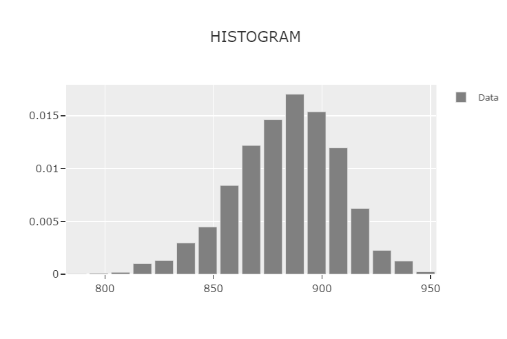
Histogram Plot
import phitter
data: list[int | float] = [...]
phitter_cont = phitter.PHITTER(data)
phitter_cont.fit()

phitter_cont.plot_histogram()
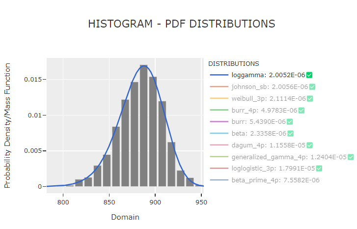
Histogram PDF Dsitributions Plot
import phitter
data: list[int | float] = [...]
phitter_cont = phitter.PHITTER(data)
phitter_cont.fit()

phitter_cont.plot_histogram_distributions()
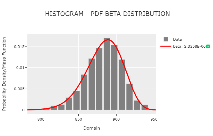
Histogram PDF Dsitribution Plot
import phitter
data: list[int | float] = [...]
phitter_cont = phitter.PHITTER(data)
phitter_cont.fit()

phitter_cont.plot_distribution("beta")
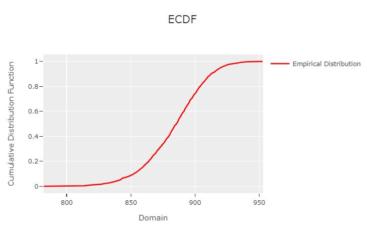
ECDF Plot
import phitter
data: list[int | float] = [...]
phitter_cont = phitter.PHITTER(data)
phitter_cont.fit()

phitter_cont.plot_ecdf()
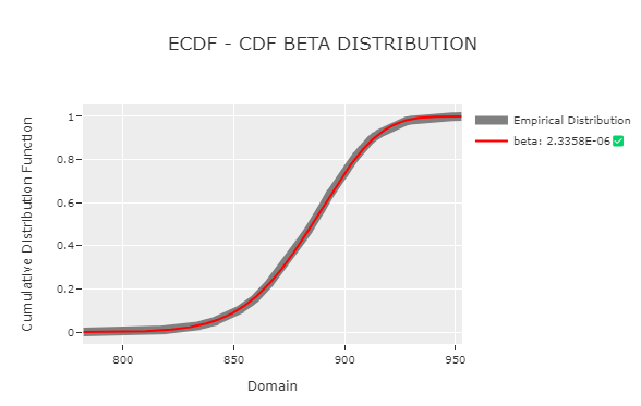
ECDF Distribution Plot
import phitter
data: list[int | float] = [...]
phitter_cont = phitter.PHITTER(data)
phitter_cont.fit()

phitter_cont.plot_ecdf_distribution("beta")
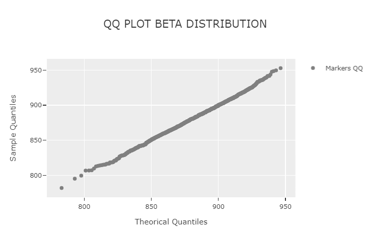
QQ Plot
import phitter
data: list[int | float] = [...]
phitter_cont = phitter.PHITTER(data)
phitter_cont.fit()

phitter_cont.qq_plot("beta")
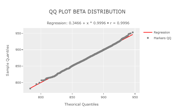
QQ - Regression Plot
import phitter
data: list[int | float] = [...]
phitter_cont = phitter.PHITTER(data)
phitter_cont.fit()

phitter_cont.qq_plot_regression("beta")
Distributions: Methods and properties
import phitter

distribution = phitter.continuous.BETA(parameters={"alpha": 5, "beta": 3, "A": 200, "B": 1000})

## CDF, PDF, PPF, PMF receive float or numpy.ndarray. For discrete distributions PMF instead of PDF. Parameters notation are in description of ditribution
distribution.cdf(752) # -> 0.6242831129533498
distribution.pdf(388) # -> 0.0002342575686629883
distribution.ppf(0.623) # -> 751.5512889417921
distribution.sample(2) # -> [550.800114   514.85410326]

## STATS
distribution.mean # -> 700.0
distribution.variance # -> 16666.666666666668
distribution.standard_deviation # -> 129.09944487358058
distribution.skewness # -> -0.3098386676965934
distribution.kurtosis # -> 2.5854545454545454
distribution.median # -> 708.707130841534
distribution.mode # -> 733.3333333333333
Continuous Distributions
1. PDF File Documentation Continuous Distributions
2. Phitter Online Interactive Documentation
Discrete Distributions
1. PDF File Documentation Discrete Distributions
2. Phitter Online Interactive Documentation
Benchmarks
Fit time continuous distributions
| Sample Size / Workers | 1 | 2 | 6 | 10 | 20 |
|---|---|---|---|---|---|
| 1K | 8.2981 | 7.1242 | 8.9667 | 9.9287 | 16.2246 |
| 10K | 20.8711 | 14.2647 | 10.5612 | 11.6004 | 17.8562 |
| 100K | 152.6296 | 97.2359 | 57.7310 | 51.6182 | 53.2313 |
| 500K | 914.9291 | 640.8153 | 370.0323 | 267.4597 | 257.7534 |
| 1M | 1580.8501 | 972.3985 | 573.5429 | 496.5569 | 425.7809 |
Estimation time parameters continuous distributions
| Sample Size / Workers | 1 | 2 | 4 |
|---|---|---|---|
| 1K | 0.1688 | 2.6402 | 2.8719 |
| 10K | 0.4462 | 2.4452 | 3.0471 |
| 100K | 4.5598 | 6.3246 | 7.5869 |
| 500K | 19.0172 | 21.8047 | 19.8420 |
| 1M | 39.8065 | 29.8360 | 30.2334 |
Estimation time parameters continuous distributions
| Distribution / Sample Size | 1K | 10K | 100K | 500K | 1M | 10M |
|---|---|---|---|---|---|---|
| alpha | 0.3345 | 0.4625 | 2.5933 | 18.3856 | 39.6533 | 362.2951 |
| arcsine | 0.0000 | 0.0000 | 0.0000 | 0.0000 | 0.0000 | 0.0000 |
| argus | 0.0559 | 0.2050 | 2.2472 | 13.3928 | 41.5198 | 362.2472 |
| beta | 0.1880 | 0.1790 | 0.1940 | 0.2110 | 0.1800 | 0.3134 |
| beta_prime | 0.1766 | 0.7506 | 7.6039 | 40.4264 | 85.0677 | 812.1323 |
| beta_prime_4p | 0.0720 | 0.3630 | 3.9478 | 20.2703 | 40.2709 | 413.5239 |
| bradford | 0.0110 | 0.0000 | 0.0000 | 0.0000 | 0.0000 | 0.0010 |
| burr | 0.0733 | 0.6931 | 5.5425 | 36.7684 | 79.8269 | 668.2016 |
| burr_4p | 0.1552 | 0.7981 | 8.4716 | 44.4549 | 87.7292 | 858.0035 |
| cauchy | 0.0090 | 0.0160 | 0.1581 | 1.1052 | 2.1090 | 21.5244 |
| chi_square | 0.0000 | 0.0000 | 0.0000 | 0.0000 | 0.0000 | 0.0000 |
| chi_square_3p | 0.0510 | 0.3545 | 3.0933 | 14.4116 | 21.7277 | 174.8392 |
| dagum | 0.3381 | 0.8278 | 9.6907 | 45.5855 | 98.6691 | 917.6713 |
| dagum_4p | 0.3646 | 1.3307 | 13.3437 | 70.9462 | 140.9371 | 1396.3368 |
| erlang | 0.0010 | 0.0000 | 0.0000 | 0.0000 | 0.0000 | 0.0000 |
| erlang_3p | 0.0000 | 0.0000 | 0.0000 | 0.0000 | 0.0000 | 0.0000 |
| error_function | 0.0000 | 0.0000 | 0.0000 | 0.0000 | 0.0000 | 0.0000 |
| exponential | 0.0000 | 0.0000 | 0.0000 | 0.0000 | 0.0000 | 0.0000 |
| exponential_2p | 0.0000 | 0.0000 | 0.0000 | 0.0000 | 0.0000 | 0.0000 |
| f | 0.0592 | 0.2948 | 2.6920 | 18.9458 | 29.9547 | 402.2248 |
| fatigue_life | 0.0352 | 0.1101 | 1.7085 | 9.0090 | 20.4702 | 186.9631 |
| folded_normal | 0.0020 | 0.0020 | 0.0020 | 0.0022 | 0.0033 | 0.0040 |
| frechet | 0.1313 | 0.4359 | 5.7031 | 39.4202 | 43.2469 | 671.3343 |
| f_4p | 0.3269 | 0.7517 | 0.6183 | 0.6037 | 0.5809 | 0.2073 |
| gamma | 0.0000 | 0.0000 | 0.0000 | 0.0000 | 0.0000 | 0.0000 |
| gamma_3p | 0.0000 | 0.0000 | 0.0000 | 0.0000 | 0.0000 | 0.0000 |
| generalized_extreme_value | 0.0833 | 0.2054 | 2.0337 | 10.3301 | 22.1340 | 243.3120 |
| generalized_gamma | 0.0298 | 0.0178 | 0.0227 | 0.0236 | 0.0170 | 0.0241 |
| generalized_gamma_4p | 0.0371 | 0.0116 | 0.0732 | 0.0725 | 0.0707 | 0.0730 |
| generalized_logistic | 0.1040 | 0.1073 | 0.1037 | 0.0819 | 0.0989 | 0.0836 |
| generalized_normal | 0.0154 | 0.0736 | 0.7367 | 2.4831 | 5.9752 | 55.2417 |
| generalized_pareto | 0.3189 | 0.8978 | 8.9370 | 51.3813 | 101.6832 | 1015.2933 |
| gibrat | 0.0328 | 0.0432 | 0.4287 | 2.7159 | 5.5721 | 54.1702 |
| gumbel_left | 0.0000 | 0.0000 | 0.0000 | 0.0000 | 0.0010 | 0.0010 |
| gumbel_right | 0.0000 | 0.0000 | 0.0000 | 0.0000 | 0.0000 | 0.0000 |
| half_normal | 0.0010 | 0.0000 | 0.0000 | 0.0010 | 0.0000 | 0.0000 |
| hyperbolic_secant | 0.0000 | 0.0000 | 0.0000 | 0.0000 | 0.0000 | 0.0000 |
| inverse_gamma | 0.0308 | 0.0632 | 0.7233 | 5.0127 | 10.7885 | 99.1316 |
| inverse_gamma_3p | 0.0787 | 0.1472 | 1.6513 | 11.1161 | 23.4587 | 227.6125 |
| inverse_gaussian | 0.0000 | 0.0000 | 0.0000 | 0.0000 | 0.0000 | 0.0000 |
| inverse_gaussian_3p | 0.0000 | 0.0000 | 0.0000 | 0.0000 | 0.0000 | 0.0000 |
| johnson_sb | 0.2966 | 0.7466 | 4.0707 | 40.2028 | 56.2130 | 728.2447 |
| johnson_su | 0.0070 | 0.0010 | 0.0010 | 0.0143 | 0.0010 | 0.0010 |
| kumaraswamy | 0.0164 | 0.0120 | 0.0130 | 0.0123 | 0.0125 | 0.0150 |
| laplace | 0.0000 | 0.0000 | 0.0000 | 0.0000 | 0.0000 | 0.0000 |
| levy | 0.0100 | 0.0314 | 0.2296 | 1.1365 | 2.7211 | 26.4966 |
| loggamma | 0.0085 | 0.0050 | 0.0050 | 0.0070 | 0.0062 | 0.0080 |
| logistic | 0.0000 | 0.0000 | 0.0000 | 0.0000 | 0.0000 | 0.0000 |
| loglogistic | 0.1402 | 0.3464 | 3.9673 | 12.0310 | 42.0038 | 471.0324 |
| loglogistic_3p | 0.2558 | 0.9152 | 11.1546 | 56.5524 | 114.5535 | 1118.6104 |
| lognormal | 0.0000 | 0.0000 | 0.0000 | 0.0000 | 0.0010 | 0.0000 |
| maxwell | 0.0000 | 0.0000 | 0.0000 | 0.0000 | 0.0000 | 0.0010 |
| moyal | 0.0000 | 0.0000 | 0.0000 | 0.0000 | 0.0000 | 0.0000 |
| nakagami | 0.0000 | 0.0030 | 0.0213 | 0.1215 | 0.2649 | 2.2457 |
| non_central_chi_square | 0.0000 | 0.0000 | 0.0000 | 0.0000 | 0.0000 | 0.0000 |
| non_central_f | 0.0190 | 0.0182 | 0.0210 | 0.0192 | 0.0190 | 0.0200 |
| non_central_t_student | 0.0874 | 0.0822 | 0.0862 | 0.1314 | 0.2516 | 0.1781 |
| normal | 0.0000 | 0.0000 | 0.0000 | 0.0000 | 0.0000 | 0.0000 |
| pareto_first_kind | 0.0010 | 0.0030 | 0.0390 | 0.2494 | 0.5226 | 5.5246 |
| pareto_second_kind | 0.0643 | 0.1522 | 1.1722 | 10.9871 | 23.6534 | 201.1626 |
| pert | 0.0052 | 0.0030 | 0.0030 | 0.0040 | 0.0040 | 0.0092 |
| power_function | 0.0075 | 0.0040 | 0.0040 | 0.0030 | 0.0040 | 0.0040 |
| rayleigh | 0.0000 | 0.0000 | 0.0000 | 0.0000 | 0.0000 | 0.0000 |
| reciprocal | 0.0000 | 0.0000 | 0.0000 | 0.0000 | 0.0000 | 0.0000 |
| rice | 0.0182 | 0.0030 | 0.0040 | 0.0060 | 0.0030 | 0.0050 |
| semicircular | 0.0000 | 0.0000 | 0.0000 | 0.0000 | 0.0000 | 0.0000 |
| trapezoidal | 0.0083 | 0.0072 | 0.0073 | 0.0060 | 0.0070 | 0.0060 |
| triangular | 0.0000 | 0.0000 | 0.0000 | 0.0000 | 0.0000 | 0.0000 |
| t_student | 0.0000 | 0.0000 | 0.0000 | 0.0000 | 0.0000 | 0.0000 |
| t_student_3p | 0.3892 | 1.1860 | 11.2759 | 71.1156 | 143.1939 | 1409.8578 |
| uniform | 0.0000 | 0.0000 | 0.0000 | 0.0000 | 0.0000 | 0.0000 |
| weibull | 0.0010 | 0.0000 | 0.0000 | 0.0000 | 0.0010 | 0.0010 |
| weibull_3p | 0.0061 | 0.0040 | 0.0030 | 0.0040 | 0.0050 | 0.0050 |
Estimation time parameters discrete distributions
| Distribution / Sample Size | 1K | 10K | 100K | 500K | 1M | 10M |
|---|---|---|---|---|---|---|
| bernoulli | 0.0000 | 0.0000 | 0.0000 | 0.0000 | 0.0000 | 0.0000 |
| binomial | 0.0000 | 0.0000 | 0.0000 | 0.0000 | 0.0000 | 0.0000 |
| geometric | 0.0000 | 0.0000 | 0.0000 | 0.0000 | 0.0000 | 0.0000 |
| hypergeometric | 0.0773 | 0.0061 | 0.0030 | 0.0020 | 0.0030 | 0.0051 |
| logarithmic | 0.0210 | 0.0035 | 0.0171 | 0.0050 | 0.0030 | 0.0756 |
| negative_binomial | 0.0293 | 0.0000 | 0.0000 | 0.0000 | 0.0000 | 0.0000 |
| poisson | 0.0000 | 0.0000 | 0.0000 | 0.0000 | 0.0000 | 0.0000 |
| uniform | 0.0000 | 0.0000 | 0.0000 | 0.0000 | 0.0000 | 0.0000 |
Contribution
If you would like to contribute to the Phitter project, please create a pull request with your proposed changes or enhancements. All contributions are welcome!


Download files
Download the file for your platform. If you're not sure which to choose, learn more about installing packages.


