`pydbm` is Python library for building Restricted Boltzmann Machine(RBM), Deep Boltzmann Machine(DBM), Recurrent neural network Restricted Boltzmann Machine(RNN-RBM), LSTM Recurrent Temporal Restricted Boltzmann Machine(LSTM-RTRBM), and Shape Boltzmann Machine(Shape-BM).


Project description
Deep Learning Library: pydbm
pydbm is Python library for building Restricted Boltzmann Machine(RBM), Deep Boltzmann Machine(DBM), Long Short-Term Memory Recurrent Temporal Restricted Boltzmann Machine(LSTM-RTRBM), and Shape Boltzmann Machine(Shape-BM).
This is Cython version. pydbm_mxnet (MXNet version) is derived from this library.
Documentation
Full documentation is available on https://code.accel-brain.com/Deep-Learning-by-means-of-Design-Pattern/ . This document contains information on functionally reusability, functional scalability and functional extensibility.
Installation
Install using pip:
pip install pydbm
Or, you can install from wheel file.
pip install https://storage.googleapis.com/accel-brain-code/Deep-Learning-by-means-of-Design-Pattern/pydbm-{X.X.X}-cp36-cp36m-linux_x86_64.whl
Source code
The source code is currently hosted on GitHub.
Python package index(PyPI)
Installers for the latest released version are available at the Python package index.
Dependencies
- numpy: v1.13.3 or higher.
- cython: v0.27.1 or higher.
Description
The function of pydbm is building and modeling Restricted Boltzmann Machine(RBM) and Deep Boltzmann Machine(DBM). The models are functionally equivalent to stacked auto-encoder. The basic function is the same as dimensions reduction(or pre-training). And this library enables you to build many functional extensions from RBM and DBM such as Recurrent Temporal Restricted Boltzmann Machine(RTRBM), Recurrent Neural Network Restricted Boltzmann Machine(RNN-RBM), Long Short-Term Memory Recurrent Temporal Restricted Boltzmann Machine(LSTM-RTRBM), and Shape Boltzmann Machine(Shape-BM).
As more usecases, RTRBM, RNN-RBM, and LSTM-RTRBM can learn dependency structures in temporal patterns such as music, natural sentences, and n-gram. RTRBM is a probabilistic time-series model which can be viewed as a temporal stack of RBMs, where each RBM has a contextual hidden state that is received from the previous RBM and is used to modulate its hidden units bias. The RTRBM can be understood as a sequence of conditional RBMs whose parameters are the output of a deterministic RNN, with the constraint that the hidden units must describe the conditional distributions. This constraint can be lifted by combining a full RNN with distinct hidden units. In terms of this possibility, RNN-RBM and LSTM-RTRBM are structurally expanded model from RTRBM that allows more freedom to describe the temporal dependencies involved.
The usecases of Shape-BM are image segmentation, object detection, inpainting and graphics. Shape-BM is the model for the task of modeling binary shape images, in that samples from the model look realistic and it can generalize to generate samples that differ from training examples.
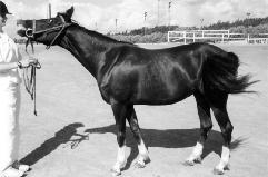
Image in the Weizmann horse dataset. |
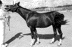
Binarized image. |
Reconstructed image by Shape-BM. |
The structure of RBM.
According to graph theory, the structure of RBM corresponds to a complete bipartite graph which is a special kind of bipartite graph where every node in the visible layer is connected to every node in the hidden layer. The state of this structure can be reflected by the energy function:
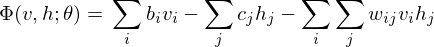
where 


The learning equations of RBM.
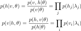
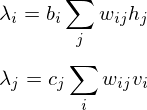
Because of the rules of conditional independence, the learning equations of RBM can be introduced as simple form. The distribution of visible state

where 


where 


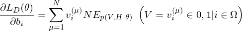
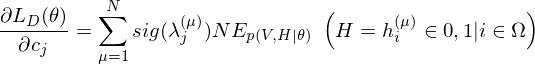
The learning equations of RBM are introduced by performing control so that those gradients can become zero.

Contrastive Divergence as an approximation method.
In relation to RBM, Contrastive Divergence(CD) is a method for approximation of the gradients of the log-likelihood. The procedure of this method is similar to Markov Chain Monte Carlo method(MCMC). However, unlike MCMC, the visbile variables to be set first in visible layer is not randomly initialized but the observed data points in training dataset are set to the first visbile variables. And, like Gibbs sampler, drawing samples from hidden variables and visible variables is repeated k times. Empirically (and surprisingly), k is considered to be 1.
The structure of DBM.
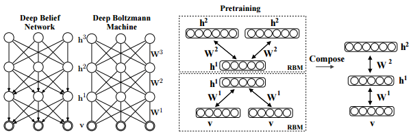
Salakhutdinov, R., Hinton, G. E. (2009). Deep boltzmann machines. In International conference on artificial intelligence and statistics (pp. 448-455). p451.
As is well known, DBM is composed of layers of RBMs stacked on top of each other. This model is a structural expansion of Deep Belief Networks(DBN), which is known as one of the earliest models of Deep Learning. Like RBM, DBN places nodes in layers. However, only the uppermost layer is composed of undirected edges, and the other consists of directed edges. DBN with R hidden layers is below probabilistic model:
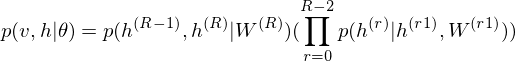
where r = 0 points to visible layer. Considerling simultaneous distribution in top two layer,

and conditional distributions in other layers are as follows:

The pre-training of DBN engages in a procedure of recursive learning in layer-by-layer. However, as you can see from the difference of graph structure, DBM is slightly different from DBN in the form of pre-training. For instance, if r = 1, the conditional distribution of visible layer is
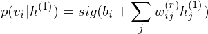 .
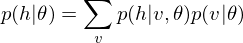
.On the other hand, the conditional distribution in the intermediate layer is
where 2 has been introduced considering that the intermediate layer r receives input data from Shallower layer
r-1 and deeper layer r+1. DBM sets these parameters as initial states.
DBM as a Stacked Auto-Encoder.
DBM is functionally equivalent to a Stacked Auto-Encoder, which is-a neural network that tries to reconstruct its input. To encode the observed data points, the function of DBM is as linear transformation of feature map below
 .
.On the other hand, to decode this feature points, the function of DBM is as linear transformation of feature map below
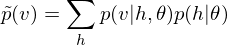 .
.The reconstruction error should be calculated in relation to problem setting. This library provides a default method, which can be overridden, for error function that computes Mean Squared Error(MSE).
Structural expansion for RTRBM.
The RTRBM (Sutskever, I., et al. 2009) is a probabilistic time-series model which can be viewed as a temporal stack of RBMs, where each RBM has a contextual hidden state that is received from the previous RBM and is used to modulate its hidden units bias. Let 
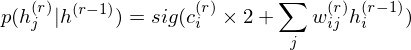
t-1. The conditional distribution in hidden layer in time t is

where 

While the hidden units are binary during inference and sampling, it is the mean-field value 

Structural expansion for RNN-RBM.
The RTRBM can be understood as a sequence of conditional RBMs whose parameters are the output of a deterministic RNN, with the constraint that the hidden units must describe the conditional distributions and convey temporal information. This constraint can be lifted by combining a full RNN with distinct hidden units. RNN-RBM (Boulanger-Lewandowski, N., et al. 2012), which is the more structural expansion of RTRBM, has also hidden units
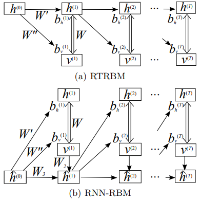
Boulanger-Lewandowski, N., Bengio, Y., & Vincent, P. (2012). Modeling temporal dependencies in high-dimensional sequences: Application to polyphonic music generation and transcription. arXiv preprint arXiv:1206.6392., p4. Single arrows represent a deterministic function, double arrows represent the stochastic hidden-visible connections of an RBM.
The biases are linear function of 
t by the relation:

where 

Structural expansion for LSTM-RTRBM.
An example of the application to polyphonic music generation(Lyu, Q., et al. 2015) clued me in on how is it possible to connect RTRBM with LSTM. LSTM-RTRBM model integrates the ability of LSTM in memorizing and retrieving useful history information, together with the advantage of RBM in high dimensional data modelling. Like RTRBM, LSTM-RTRBM also has the recurrent hidden units. Let 

where 

"Adding LSTM units to RTRBM is not trivial, considering RTRBM’s hidden units and visible units are intertwined in inference and learning. The simplest way to circumvent this difficulty is to use bypass connections from LSTM units to the hidden units besides the existing recurrent connections of hidden units, as in LSTM-RTRBM."
Therefore it is useful to introduce a distinction of channel which means the sequential information. 


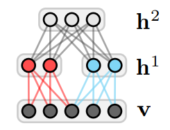
Structural expansion for Shape-BM.
The concept of Shape Boltzmann Machine (Eslami, S. A., et al. 2014) provided inspiration to this library. This model uses below has two layers of hidden variables: 

v arethe pixels of a binary image of size 


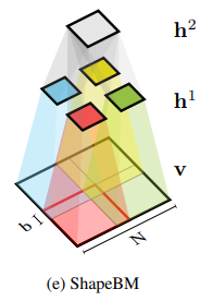
Eslami, S. A., Heess, N., Williams, C. K., & Winn, J. (2014). The shape boltzmann machine: a strong model of object shape. International Journal of Computer Vision, 107(2), 155-176., p156. |
Eslami, S. A., Heess, N., Williams, C. K., & Winn, J. (2014). The shape boltzmann machine: a strong model of object shape. International Journal of Computer Vision, 107(2), 155-176., p156. |
The Shape-BM is a DBM in three layer. The learning algorithm can be completed by optimization of

where 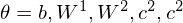
The commonality/variability analysis in order to practice object-oriented design.
From perspective of commonality/variability analysis in order to practice object-oriented design, the concepts of RBM and DBM paradigms can be organized as follows.
While each model is common in that it is constituted by stacked RBM, its approximation methods and activation functions are variable depending on the problem settings. Considering the commonality, it is useful to design based on Builder Pattern, which separates the construction of RBM object from its representation so that the same construction process can create different representations such as DBM, RTRBM, RNN-RBM, and Shape-BM. On the other hand, to deal with the variability, Strategy Pattern, which provides a way to define a family of algorithms such as approximation methods and activation functions, is useful design method, which is encapsulate each one as an object, and make them interchangeable from the point of view of functionally equivalent.
Usecase: Building the deep boltzmann machine for feature extracting.
Import Python and Cython modules.
# The `Client` in Builder Pattern
from pydbm.dbm.deep_boltzmann_machine import DeepBoltzmannMachine
# The `Concrete Builder` in Builder Pattern.
from pydbm.dbm.builders.dbm_multi_layer_builder import DBMMultiLayerBuilder
# Contrastive Divergence for function approximation.
from pydbm.approximation.contrastive_divergence import ContrastiveDivergence
# Logistic Function as activation function.
from pydbm.activation.logistic_function import LogisticFunction
# Tanh Function as activation function.
from pydbm.activation.tanh_function import TanhFunction
# ReLu Function as activation function.
from pydbm.activation.relu_function import ReLuFunction
Instantiate objects and call the method.
dbm = DeepBoltzmannMachine(
    DBMMultiLayerBuilder(),
    # Dimention in visible layer, hidden layer, and second hidden layer.
    [train_arr.shape[1], 10, train_arr.shape[1]],
    # Setting objects for activation function.
    [ReLuFunction(), LogisticFunction(), TanhFunction()],
    # Setting the object for function approximation.
    [ContrastiveDivergence(), ContrastiveDivergence()],
    # Setting learning rate.
    0.05,
    # Setting dropout rate.
    0.5
)

# Execute learning.
dbm.learn(
    train_arr,
     # If approximation is the Contrastive Divergence, this parameter is `k` in CD method.
    training_count=1,
    # Batch size in mini-batch training.
    batch_size=200,
    # if `r_batch_size` > 0, the function of `dbm.learn` is a kind of reccursive learning.
    r_batch_size=-1
)
If you do not want to execute the mini-batch training, the value of batch_size must be -1. And r_batch_size is also parameter to control the mini-batch training but is refered only in inference and reconstruction. If this value is more than 0, the inferencing is a kind of reccursive learning with the mini-batch training.
And the feature points can be extracted by this method.
print(dbm.get_feature_point(layer_number=1))
Usecase: Extracting all feature points for dimensions reduction(or pre-training)
Import Python and Cython modules.
# `StackedAutoEncoder` is-a `DeepBoltzmannMachine`.
from pydbm.dbm.deepboltzmannmachine.stacked_auto_encoder import StackedAutoEncoder
# The `Concrete Builder` in Builder Pattern.
from pydbm.dbm.builders.dbm_multi_layer_builder import DBMMultiLayerBuilder
# Contrastive Divergence for function approximation.
from pydbm.approximation.contrastive_divergence import ContrastiveDivergence
# Logistic Function as activation function.
from pydbm.activation.logistic_function import LogisticFunction
Instantiate objects and call the method.
# Setting objects for activation function.
activation_list = [LogisticFunction(), LogisticFunction(), LogisticFunction()]
# Setting the object for function approximation.
approximaion_list = [ContrastiveDivergence(), ContrastiveDivergence()]

dbm = StackedAutoEncoder(
    DBMMultiLayerBuilder(),
    [target_arr.shape[1], 10, target_arr.shape[1]],
    activation_list,
    approximaion_list,
    0.05, # Setting learning rate.
    0.5   # Setting dropout rate.
)

# Execute learning.
dbm.learn(
    target_arr,
    1, # If approximation is the Contrastive Divergence, this parameter is `k` in CD method.
    batch_size=200,  # Batch size in mini-batch training.
    r_batch_size=-1  # if `r_batch_size` > 0, the function of `dbm.learn` is a kind of reccursive learning.
)
Extract reconstruction error rate.
You can check the reconstruction error rate. During the approximation of the Contrastive Divergence, the mean squared error(MSE) between the observed data points and the activities in visible layer is computed as the reconstruction error rate.
Call get_reconstruct_error_arr method as follow.
reconstruct_error_arr = dbm.get_reconstruct_error_arr(layer_number=0)
layer_number corresponds to the index of approximaion_list. And reconstruct_error_arr is the np.ndarray of reconstruction error rates.
Extract the result of dimention reduction
And the result of dimention reduction can be extracted by this property.
pre_trained_arr = dbm.feature_points_arr
Extract weights obtained by pre-training.
If you want to get the pre-training weights, call get_weight_arr_list method.
weight_arr_list = dbm.get_weight_arr_list()
weight_arr_list is the list of weights of each links in DBM. weight_arr_list[0] is 2-d np.ndarray of weights between visible layer and first hidden layer.
Extract biases obtained by pre-training.
Call get_visible_bias_arr_list method and get_hidden_bias_arr_list method in the same way.
visible_bias_arr_list = dbm.get_visible_bias_arr_list()
hidden_bias_arr_list = dbm.get_hidden_bias_arr_list()
visible_bias_arr_list and hidden_bias_arr_list are the list of biases of each links in DBM.
Transfer learning in DBM.
DBMMultiLayerBuilder can be given weight_arr_list, visible_bias_arr_list, and hidden_bias_arr_list obtained by pre-training.
dbm = StackedAutoEncoder(
    DBMMultiLayerBuilder(
        # Setting pre-learned weights matrix.
        weight_arr_list,
        # Setting pre-learned bias in visible layer.
        visible_bias_arr_list,
        # Setting pre-learned bias in hidden layer.
        hidden_bias_arr_list
    ),
    [next_target_arr.shape[1], 10, next_target_arr.shape[1]],
    activation_list,
    approximaion_list,
    # Setting learning rate.
    0.05,
    # Setting dropout rate.
    0.0
)

# Execute learning.
dbm.learn(
    next_target_arr,
    1, # If approximation is the Contrastive Divergence, this parameter is `k` in CD method.
    batch_size=200,  # Batch size in mini-batch training.
    r_batch_size=-1  # if `r_batch_size` > 0, the function of `dbm.learn` is a kind of reccursive learning.
)
Performance
Run a program: demo_stacked_auto_encoder.py
time python demo_stacked_auto_encoder.py
The result is follow.
real    1m35.472s
user    1m32.300s
sys     0m3.136s
Detail
This experiment was performed under the following conditions.
Machine type
- vCPU:
2 - memory:
8GB - CPU Platform: Intel Ivy Bridge
Observation Data Points
The observated data is the result of np.random.uniform(size=(10000, 10000)).
Number of units
- Visible layer:
10000 - hidden layer(feature point):
10 - hidden layer:
10000
Activation functions
- visible: Logistic Function
- hidden(feature point): Logistic Function
- hidden: Logistic Function
Approximation
- Contrastive Divergence
Hyper parameters
- Learning rate:
0.05 - Dropout rate:
0.5
Feature points
0.190599  0.183594  0.482996  0.911710  0.939766  0.202852  0.042163
0.470003  0.104970  0.602966  0.927917  0.134440  0.600353  0.264248
0.419805  0.158642  0.328253  0.163071  0.017190  0.982587  0.779166
0.656428  0.947666  0.409032  0.959559  0.397501  0.353150  0.614216
0.167008  0.424654  0.204616  0.573720  0.147871  0.722278  0.068951
.....
Reconstruct error
[ 0.08297197 0.07091231 0.0823424 ..., 0.0721624 0.08404181 0.06981017]
Usecase: Building the RTRBM for recursive learning.
Import Python and Cython modules.
# `Builder` in `Builder Patter`.
from pydbm.dbm.builders.rt_rbm_simple_builder import RTRBMSimpleBuilder
# RNN and Contrastive Divergence for function approximation.
from pydbm.approximation.rt_rbm_cd import RTRBMCD
# Logistic Function as activation function.
from pydbm.activation.logistic_function import LogisticFunction
# Softmax Function as activation function.
from pydbm.activation.softmax_function import SoftmaxFunction
Instantiate objects and execute learning.
# `Builder` in `Builder Pattern` for RTRBM.
rtrbm_builder = RTRBMSimpleBuilder()
# Learning rate.
rtrbm_builder.learning_rate = 0.00001
# Set units in visible layer.
rtrbm_builder.visible_neuron_part(LogisticFunction(), arr.shape[1])
# Set units in hidden layer.
rtrbm_builder.hidden_neuron_part(LogisticFunction(), 3)
# Set units in RNN layer.
rtrbm_builder.rnn_neuron_part(LogisticFunction())
# Set graph and approximation function.
rtrbm_builder.graph_part(RTRBMCD())
# Building.
rbm = rtrbm_builder.get_result()

# Learning.
rbm.learn(
    arr,
    training_count=1,
    batch_size=200
)
The rbm has a np.ndarray of graph.visible_activity_arr. The graph.visible_activity_arr is the inferenced feature points. This value can be observed as data point.
# Execute recursive learning.
inferenced_arr = rbm.inference(
    test_arr,
    training_count=1,
    r_batch_size=-1
)
Returned value inferenced_arr is generated by input parameter test_arr.
Usecase: Building the RNN-RBM for recursive learning.
Import Python and Cython modules.
# `Builder` in `Builder Patter`.
from pydbm.dbm.builders.rnn_rbm_simple_builder import RNNRBMSimpleBuilder
# RNN and Contrastive Divergence for function approximation.
from pydbm.approximation.rtrbmcd.rnn_rbm_cd import RNNRBMCD
# Logistic Function as activation function.
from pydbm.activation.logistic_function import LogisticFunction
# Softmax Function as activation function.
from pydbm.activation.softmax_function import SoftmaxFunction
Instantiate objects.
# `Builder` in `Builder Pattern` for RNN-RBM.
rnnrbm_builder = RNNRBMSimpleBuilder()
# Learning rate.
rnnrbm_builder.learning_rate = 0.00001
# Set units in visible layer.
rnnrbm_builder.visible_neuron_part(LogisticFunction(), arr.shape[1])
# Set units in hidden layer.
rnnrbm_builder.hidden_neuron_part(LogisticFunction(), 3)
# Set units in RNN layer.
rnnrbm_builder.rnn_neuron_part(LogisticFunction())
# Set graph and approximation function.
rnnrbm_builder.graph_part(RNNRBMCD())
# Building.
rbm = rnnrbm_builder.get_result()
The function of learning and inferencing is equivalent to rbm of RTRBM.
Usecase: Building the LSTM-RTRBM for recursive learning.
Import Python and Cython modules.
# `Builder` in `Builder Patter`.
from pydbm.dbm.builders.lstm_rt_rbm_simple_builder import LSTMRTRBMSimpleBuilder
# LSTM and Contrastive Divergence for function approximation.
from pydbm.approximation.rtrbmcd.lstm_rt_rbm_cd import LSTMRTRBMCD
# Logistic Function as activation function.
from pydbm.activation.logistic_function import LogisticFunction
# Tanh Function as activation function.
from pydbm.activation.tanh_function import TanhFunction
Instantiate objects.
# `Builder` in `Builder Pattern` for LSTM-RTRBM.
rnnrbm_builder = LSTMRTRBMSimpleBuilder()
# Learning rate.
rnnrbm_builder.learning_rate = 1e-05
# Set units in visible layer.
rnnrbm_builder.visible_neuron_part(LogisticFunction(), 50)
# Set units in hidden layer.
rnnrbm_builder.hidden_neuron_part(LogisticFunction(), 100)
# Set units in RNN layer.
rnnrbm_builder.rnn_neuron_part(TanhFunction())
# Set graph and approximation function.
rnnrbm_builder.graph_part(LSTMRTRBMCD())
# Building.
rbm = rnnrbm_builder.get_result()
The function of learning and inferencing is equivalent to rbm of RTRBM.
Usecase: Image segmentation by Shape-BM.
First, acquire image data and binarize it.
from PIL import Image
img = Image.open("horse099.jpg")
img
If you think the size of your image datasets may be large, resize it to an arbitrary size.
img = img.resize((90, 90))
Convert RGB images to binary images.
img_bin = img.convert("1")
img_bin
Set up hyperparameters.
filter_size = 5
overlap_n = 4

learning_rate = 0.01
filter_size is the 'filter' size. This value must be more than 4. And overlap_n is hyperparameter specific to Shape-BM. In the visible layer, this model has so-called local receptive fields by connecting each first hidden unit only to a subset of the visible units, corresponding to one of four square patches. Each patch overlaps its neighbor by overlap_n pixels (Eslami, S. A., et al, 2014).
Please note that the recommended ratio of filter_size and overlap_n is 5:4. It is not a constraint demanded by pure theory of Shape Boltzmann Machine itself but is a kind of limitation to simplify design and implementation in this library.
And import Python and Cython modules.
# The `Client` in Builder Pattern
from pydbm.dbm.deepboltzmannmachine.shape_boltzmann_machine import ShapeBoltzmannMachine
# The `Concrete Builder` in Builder Pattern.
from pydbm.dbm.builders.dbm_multi_layer_builder import DBMMultiLayerBuilder
Instantiate objects and call the method.
dbm = ShapeBoltzmannMachine(
    DBMMultiLayerBuilder(),
    learning_rate=learning_rate,
    overlap_n=overlap_n,
    filter_size=filter_size
)

img_arr = np.asarray(img_bin)
img_arr = img_arr.astype(np.float64)

# Execute learning.
dbm.learn(
    # `np.ndarray` of image data.
    img_arr,
    # If approximation is the Contrastive Divergence, this parameter is `k` in CD method.
    training_count=1,
    # Batch size in mini-batch training.
    batch_size=300,
    # if `r_batch_size` > 0, the function of `dbm.learn` is a kind of reccursive learning.
    r_batch_size=-1,
    # Learning with the stochastic gradient descent(SGD) or not.
    sgd_flag=True
)
Extract dbm.visible_points_arr as the observed data points in visible layer. This np.ndarray is segmented image data.
inferenced_data_arr = dbm.visible_points_arr.copy()
inferenced_data_arr = 255 - inferenced_data_arr
Image.fromarray(np.uint8(inferenced_data_arr))
References
- Ackley, D. H., Hinton, G. E., & Sejnowski, T. J. (1985). A learning algorithm for Boltzmann machines. Cognitive science, 9(1), 147-169.
- Boulanger-Lewandowski, N., Bengio, Y., & Vincent, P. (2012). Modeling temporal dependencies in high-dimensional sequences: Application to polyphonic music generation and transcription. arXiv preprint arXiv:1206.6392.
- Eslami, S. A., Heess, N., Williams, C. K., & Winn, J. (2014). The shape boltzmann machine: a strong model of object shape. International Journal of Computer Vision, 107(2), 155-176.
- Hinton, G. E. (2002). Training products of experts by minimizing contrastive divergence. Neural computation, 14(8), 1771-1800.
- Le Roux, N., & Bengio, Y. (2008). Representational power of restricted Boltzmann machines and deep belief networks. Neural computation, 20(6), 1631-1649.
- Lyu, Q., Wu, Z., Zhu, J., & Meng, H. (2015, June). Modelling High-Dimensional Sequences with LSTM-RTRBM: Application to Polyphonic Music Generation. In IJCAI (pp. 4138-4139).
- Lyu, Q., Wu, Z., & Zhu, J. (2015, October). Polyphonic music modelling with LSTM-RTRBM. In Proceedings of the 23rd ACM international conference on Multimedia (pp. 991-994). ACM.
- Salakhutdinov, R., & Hinton, G. E. (2009). Deep boltzmann machines. InInternational conference on artificial intelligence and statistics (pp. 448-455).
- Srivastava, N., Hinton, G., Krizhevsky, A., Sutskever, I., & Salakhutdinov, R. (2014). Dropout: a simple way to prevent neural networks from overfitting. The Journal of Machine Learning Research, 15(1), 1929-1958.
- Sutskever, I., Hinton, G. E., & Taylor, G. W. (2009). The recurrent temporal restricted boltzmann machine. In Advances in Neural Information Processing Systems (pp. 1601-1608).
- Zaremba, W., Sutskever, I., & Vinyals, O. (2014). Recurrent neural network regularization. arXiv preprint arXiv:1409.2329.
More detail demos
- Webクローラ型人工知能:キメラ・ネットワークの仕様 (Japanese)
- Implemented by the
C++version of this library, these 20001 bots are able to execute the dimensions reduction(or pre-training) for natural language processing to run as 20001 web-crawlers and 20001 web-scrapers.
- Implemented by the
- ハッカー倫理に準拠した人工知能のアーキテクチャ設計 (Japanese)
Related PoC
- Webクローラ型人工知能によるパラドックス探索暴露機能の社会進化論 (Japanese)
- 深層強化学習のベイズ主義的な情報探索に駆動された自然言語処理の意味論 (Japanese)
- ハッカー倫理に準拠した人工知能のアーキテクチャ設計 (Japanese)
- ヴァーチャルリアリティにおける動物的「身体」の物神崇拝的なユースケース (Japanese)
Author
- chimera0(RUM)
Author URI
License
- GNU General Public License v2.0
Release history Release notifications | RSS feed


Download files
Download the file for your platform. If you're not sure which to choose, learn more about installing packages.


