pyqlearning is Python library to implement Reinforcement Learning, especially for Q-Learning.


Project description
Reinforcement Learning Library: pyqlearning
pyqlearning is Python library to implement Reinforcement Learning, especially for Q-Learning.
Installation
Install using pip:
pip install pyqlearning
Source code
The source code is currently hosted on GitHub.
Python package index(PyPI)
Installers for the latest released version are available at the Python package index.
Dependencies
- numpy: v1.13.3 or higher.
- pandas: v0.22.0 or higher.
Description
In Reinforcement Learning problem settings, Q-Learning is a kind of Temporal Difference learning(TD Learning) that can be considered as hybrid of Monte Carlo method and Dynamic Programming Method. As Monte Carlo method, TD Learning algorithm can learn by experience without model of environment. And this learning algorithm is functional extension of bootstrap method as Dynamic Programming Method.
In this library, Q-Learning can be distinguished into Epsilon Greedy Q-Leanring and Boltzmann Q-Learning. These algorithm is functionally equivalent but their structures should be conceptually distinguished.
Epsilon Greedy Q-Leanring algorithm is a typical off-policy algorithm. In this paradigm, stochastic searching and deterministic searching can coexist by hyperparameter 
Boltzmann Q-Learning algorithm is based on Boltzmann action selection mechanism, where the probability


where the temperature 


Considering many variable parts and functional extensions in the Q-learning paradigm from perspective of commonality/variability analysis in order to practice object-oriented design, this library provides abstract class that defines the skeleton of a Q-Learning algorithm in an operation, deferring some steps in concrete variant algorithms such as Epsilon Greedy Q-Leanring and Boltzmann Q-Learning to client subclasses. The abstract class in this library lets subclasses redefine certain steps of a Q-Learning algorithm without changing the algorithm's structure.
Documentation
Full documentation is available on https://code.accel-brain.com/Reinforcement-Learning/ . This document contains information on functionally reusability, functional scalability and functional extensibility.
Tutorial: Simple Maze Solving by Q-Learning (Jupyter notebook)
search_maze_by_q_learning.ipynb is a Jupyter notebook which demonstrates a simple maze solving algorithm based on Epsilon-Greedy Q-Learning or Q-Learning, loosely coupled with Deep Boltzmann Machine(DBM).
In this demonstration, let me cite the Q-Learning, loosely coupled with Deep Boltzmann Machine (DBM). As API Documentation of pydbm library has pointed out, DBM is functionally equivalent to stacked auto-encoder. The main function I observe is the same as dimensions reduction(or pre-training). Then the function of this DBM is dimensionality reduction of reward value matrix.
Q-Learning, loosely coupled with Deep Boltzmann Machine (DBM), is a more effective way to solve maze. The pre-training by DBM allow Q-Learning agent to abstract feature of reward value matrix and to observe the map in a bird's-eye view. Then agent can reach the goal with a smaller number of trials.
As shown in the below image, the state-action value function and parameters setting can be designed to correspond with the optimality of route.
Maze map |
Feature Points in the maze map |
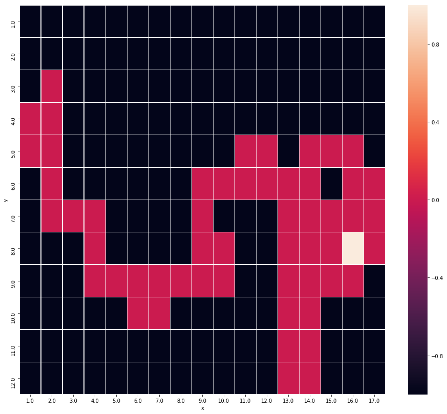
The result of searching by Epsilon-Greedy Q-Learning |
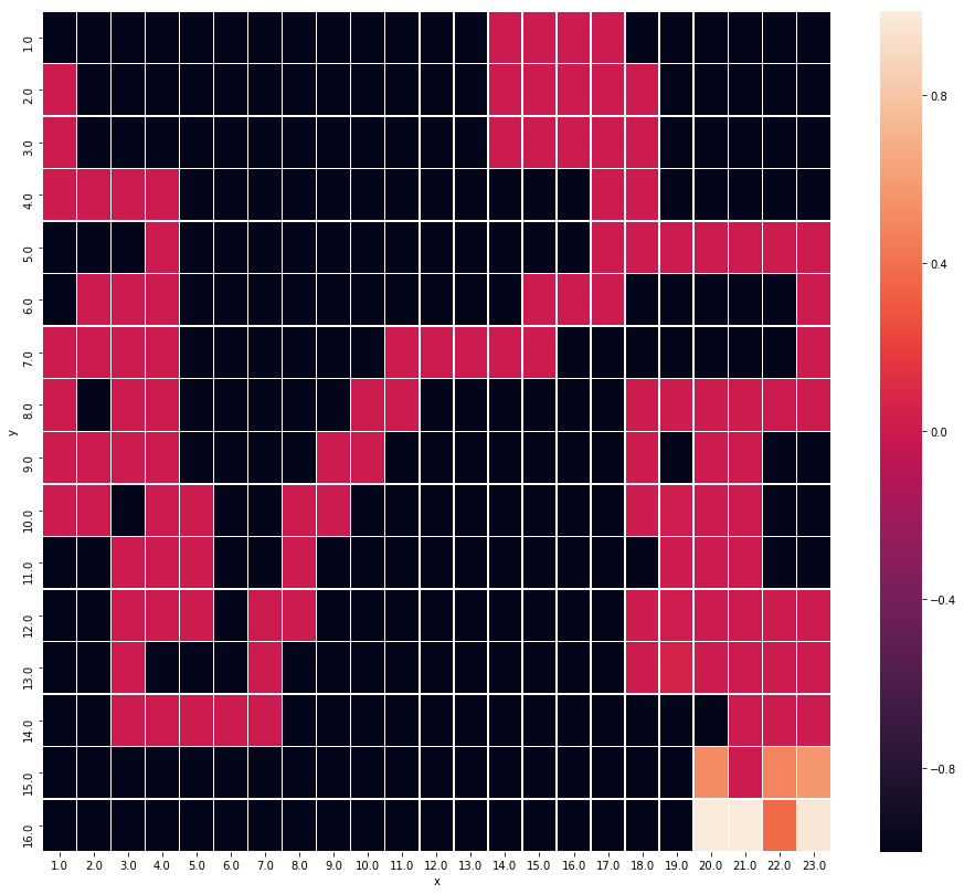
The result of searching by Q-Learning, loosely coupled with Deep Boltzmann Machine. |
Tutorial: Complexity of Hyperparameters, or how can be hyperparameters decided?
There are many hyperparameters that we have to set before the actual searching and learning process begins. Each parameter should be decided in relation to Reinforcement Learning theory and it cause side effects in training model. Because of this complexity of hyperparameters, so-called the hyperparameter tuning must become a burden of Data scientists and R & D engineers from the perspective of not only a theoretical point of view but also implementation level.
This issue can be considered as Combinatorial optimization problem which is an optimization problem, where an optimal solution has to be identified from a finite set of solutions. The solutions are normally discrete or can be converted into discrete. This is an important topic studied in operations research such as software engineering, artificial intelligence(AI), and machine learning. For instance, travelling sales man problem is one of the popular combinatorial optimization problem.
In this problem setting, this library provides an Annealing Model to search optimal combination of hyperparameters. For instance, Simulated Annealing is a probabilistic single solution based search method inspired by the annealing process in metallurgy. Annealing is a physical process referred to as tempering certain alloys of metal, glass, or crystal by heating above its melting point, holding its temperature, and then cooling it very slowly until it solidifies into a perfect crystalline structure. The simulation of this process is known as simulated annealing.
annealing_hand_written_digits.ipynb is a Jupyter notebook which demonstrates a very simple classification problem: Recognizing hand-written digits, in which the aim is to assign each input vector to one of a finite number of discrete categories, to learn observed data points from already labeled data how to predict the class of unlabeled data. In the usecase of hand-written digits dataset, the task is to predict, given an image, which digit it represents.
Demonstration: Epsilon Greedy Q-Learning and Simulated Annealing.
Import python modules.
from pyqlearning.annealingmodel.costfunctionable.greedy_q_learning_cost import GreedyQLearningCost
from pyqlearning.annealingmodel.simulated_annealing import SimulatedAnnealing
from devsample.maze_greedy_q_learning import MazeGreedyQLearning
The class GreedyQLearningCost is implemented the interface CostFunctionable to be called by AnnealingModel. This cost function is defined by
where 
Like Monte Carlo method, let us draw random samples from a normal (Gaussian) or unifrom distribution.
# Epsilon-Greedy rate in Epsilon-Greedy-Q-Learning.
greedy_rate_arr = np.random.normal(loc=0.5, scale=0.1, size=100)
# Alpha value in Q-Learning.
alpha_value_arr = np.random.normal(loc=0.5, scale=0.1, size=100)
# Gamma value in Q-Learning.
gamma_value_arr = np.random.normal(loc=0.5, scale=0.1, size=100)
# Limit of the number of Learning(searching).
limit_arr = np.random.normal(loc=10, scale=1, size=100)

cost_arr = np.c_[greedy_rate_arr, alpha_value_arr, gamma_value_arr, limit_arr]
Instantiate and initialize MazeGreedyQLearning which is-a GreedyQLearning.
# Instantiation.
greedy_q_learning = MazeGreedyQLearning()
greedy_q_learning.initialize(hoge=fuga)
Instantiate GreedyQLearningCost which is implemented the interface CostFunctionable to be called by AnnealingModel.
init_state_key = ("Some", "data")
cost_functionable = GreedyQLearningCost(
    greedy_q_learning,
    init_state_key=init_state_key
)
Instantiate SimulatedAnnealing which is-a AnnealingModel.
annealing_model = SimulatedAnnealing(
    # is-a `CostFunctionable`.
    cost_functionable=cost_functionable,
    # The number of searching cycles.
    cycles_num=5,
    # The number of trials per a cycle.
    trials_per_cycle=3
)
Fit the cost_arr to annealing_model.
annealing_model.fit_dist_mat(cost_arr)
Start annealing.
annealing_model.annealing()
To extract result of searching, call the property predicted_log_list which is list of tuple: (Cost, Delta energy, Mean of delta energy, probability in Boltzmann distribution, accept flag). And refer the property x which is np.ndarray that has combination of hyperparameters. The optimal combination can be extracted as follow.
# Extract list: [(Cost, Delta energy, Mean of delta energy, probability, accept)]
predicted_log_list = annealing_model.predicted_log_list
predicted_log_arr = np.array(predicted_log_list)

# [greedy rate, Alpha value, Gamma value, Limit of the number of searching.]
min_e_v_arr = annealing_model.x[np.argmin(predicted_log_arr[:, 2])]
Contingency of definitions
The above definition of cost function is possible option: not necessity but contingent from the point of view of modal logic. You should questions the necessity of definition and re-define, for designing the implementation of interface CostFunctionable, in relation to your problem settings.
Experiment: Q-Learning VS Q-Learning, loosely coupled with Deep Boltzmann Machine.
The tutorial in search_maze_by_q_learning.ipynb exemplifies the function of Deep Boltzmann Machine(DBM). Here, I verify if that DBM impacts on the number of searches by Q-Learning in the maze problem setting.
Batch program for Q-Learning.
demo_maze_greedy_q_learning.py is a simple maze solving algorithm. MazeGreedyQLearning in devsample/maze_greedy_q_learning.py is a Concrete Class in Template Method Pattern to run the Q-Learning algorithm for this task. GreedyQLearning in pyqlearning/qlearning/greedy_q_learning.py is also Concreat Class for the epsilon-greedy-method. The Abstract Class that defines the skeleton of Q-Learning algorithm in the operation and declares algorithm placeholders is pyqlearning/q_learning.py. So demo_maze_greedy_q_learning.py is a kind of Client in Template Method Pattern.
This algorithm allow the agent to search the goal in maze by reward value in each point in map.
The following is an example of map.
[['#' '#' '#' '#' '#' '#' '#' '#' '#' '#']
 ['#' 'S'  4   8   8   4   9   6   0  '#']
 ['#'  2  26   2   5   9   0   6   6  '#']
 ['#'  2  '@' 38   5   8   8   1   2  '#']
 ['#'  3   6   0  49   8   3   4   9  '#']
 ['#'  9   7   4   6  55   7   0   3  '#']
 ['#'  1   8   4   8   2  69   8   2  '#']
 ['#'  1   0   2   1   7   0  76   2  '#']
 ['#'  2   8   0   1   4   7   5  'G' '#']
 ['#' '#' '#' '#' '#' '#' '#' '#' '#' '#']]
#is wall in maze.Sis a start point.Gis a goal.@is the agent.
In relation to reinforcement learning theory, the state of agent is 2D position coordinates and the action is to dicide the direction of movement. Within the wall, the agent is movable in a cross direction and can advance by one point at a time. After moving into a new position, the agent can obtain a reward. On greedy searching, this extrinsically motivated agent performs in order to obtain some reward as high as possible. Each reward value is plot in map.
To see how agent can search and rearch the goal, run the batch program: demo_maze_greedy_q_learning.py
python demo_maze_greedy_q_learning.py
Batch program for Q-Learning, loosely coupled with Deep Boltzmann Machine.
demo_maze_deep_boltzmann_q_learning.py is a demonstration of how the Q-Learning can be to deepen. A so-called Deep Q-Network (DQN) is meant only as an example. In this demonstration, let me cite the Q-Learning , loosely coupled with Deep Boltzmann Machine (DBM). As API Documentation of pydbm library has pointed out, DBM is functionally equivalent to stacked auto-encoder. The main function I observe is the same as dimensions reduction(or pre-training). Then the function this DBM is dimensionality reduction of reward value matrix.
Q-Learning, loosely coupled with Deep Boltzmann Machine (DBM), is a more effective way to solve maze. The pre-training by DBM allow Q-Learning agent to abstract feature of reward value matrix and to observe the map in a bird's-eye view. Then agent can reache the goal with a smaller number of trials.
To realize the power of DBM, I performed a simple experiment.
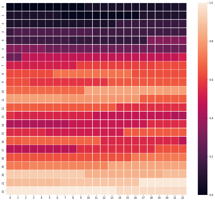
Feature engineering
For instance, a feature in each coordinate can be transformed and extracted by reward value as so-called observed data points in its adjoining points. More formally, see search_maze_by_q_learning.ipynb.
Then the feature representation can be as calculated. After this pre-training, the DBM has extracted feature points below.
[['#' '#' '#' '#' '#' '#' '#' '#' '#' '#']
 ['#' 'S' 0.22186305563593528 0.22170599483791015 0.2216928599218454
  0.22164807496640074 0.22170371283788584 0.22164021608623224
  0.2218165339471332 '#']
 ['#' 0.22174745260072407 0.221880094307873 0.22174244728061343
  0.2214709292493749 0.22174626768015263 0.2216756589222596
  0.22181057818975275 0.22174525714311788 '#']
 ['#' 0.22177496678085065 0.2219122743656551 0.22187543599733664
  0.22170745588799798 0.2215226084843615 0.22153827385193636
  0.22168466277729898 0.22179391402965035 '#']
 ['#' 0.2215341770250964 0.22174315536140118 0.22143149966676515
  0.22181685688674144 0.22178215385805333 0.2212249704384472
  0.22149210148879617 0.22185413678274837 '#']
 ['#' 0.22162363223483128 0.22171313373253035 0.2217109987501002
  0.22152432841656014 0.22175562457887335 0.22176040052504634
  0.22137688854285298 0.22175365642579478 '#']
 ['#' 0.22149515807715153 0.22169199881701832 0.22169558478042856
  0.2216904005450013 0.22145368271014734 0.2217144069625017
  0.2214896100292738 0.221398594191006 '#']
 ['#' 0.22139837944992058 0.22130176116356184 0.2215414328019404
  0.22146667964656613 0.22164354506366127 0.22148685616333666
  0.22162822887193126 0.22140174437162474 '#']
 ['#' 0.22140060918518528 0.22155145714201702 0.22162929776464463
  0.22147466752374162 0.22150300682310872 0.22162775291471243
  0.2214233075299188 'G' '#']
 ['#' '#' '#' '#' '#' '#' '#' '#' '#' '#']]
To see how agent can search and rearch the goal, install pydbm library and run the batch program: demo_maze_deep_boltzmann_q_learning.py
python demo_maze_deep_boltzmann_q_learning.py
Case 1: for more greedy searches
Map setting.
- map size:
20*20. - Start Point: (1, 1)
- End Point: (18, 18)
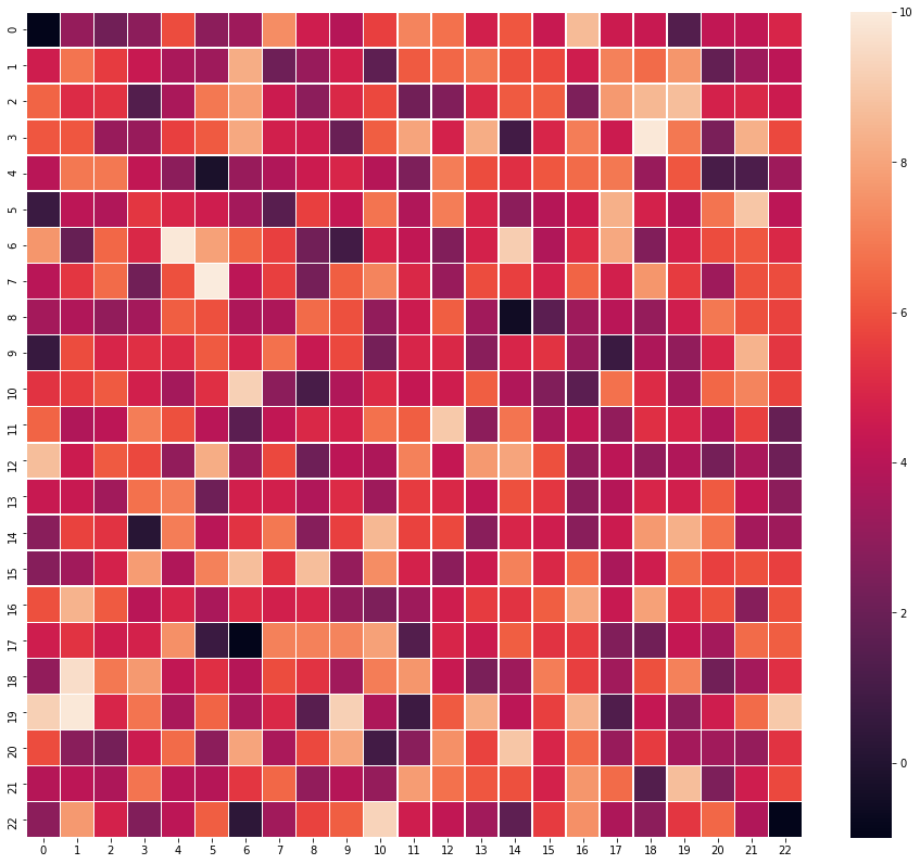
Reward value
import numpy as np

map_d = 20
map_arr = np.random.rand(map_d, map_d)
map_arr += np.diag(list(range(map_d)))
Hyperparameters
- Alpha:
0.9 - Gamma:
0.9 - Greedy rate(epsilon):
0.75- More Greedy.
Searching plan
- number of trials:
1000 - Maximum Number of searches:
10000
Metrics (Number of searches)
Tests show that the number of searches on the Q-Learning with pre-training is smaller than not with pre-training.
| Number of searches | not pre-training | pre-training |
|---|---|---|
| Max | 8155 | 4373 |
| mean | 3753.80 | 1826.0 |
| median | 3142.0 | 1192.0 |
| min | 1791 | 229 |
| var | 3262099.36 | 2342445.78 |
| std | 1806.13 | 1530.56 |
Case 2: for less greedy searches
Map setting
- map size:
20*20. - Start Point: (1, 1)
- End Point: (18, 18)
Reward value
import numpy as np

map_d = 20
map_arr = np.random.rand(map_d, map_d)
map_arr += np.diag(list(range(map_d)))
Hyperparameters
- Alpha:
0.9 - Gamma:
0.9 - Greedy rate(epsilon):
0.25- Less Greedy.
Searching plan
- number of trials:
1000 - Maximum Number of searches:
10000
Metrics (Number of searches)
| Number of searches | not pre-training | pre-training |
|---|---|---|
| Max | 10000 | 10000 |
| mean | 7136.0 | 3296.89 |
| median | 9305.0 | 1765.0 |
| min | 2401 | 195 |
| var | 9734021.11 | 10270136.10 |
| std | 3119.94 | 3204.71 |
Under the assumption that the less number of searches the better, Q-Learning, loosely coupled with Deep Boltzmann Machine, is a more effective way to solve maze in not greedy mode as well as greedy mode.
References
- Agrawal, S., & Goyal, N. (2011). Analysis of Thompson sampling for the multi-armed bandit problem. arXiv preprint arXiv:1111.1797.
- Bubeck, S., & Cesa-Bianchi, N. (2012). Regret analysis of stochastic and nonstochastic multi-armed bandit problems. arXiv preprint arXiv:1204.5721.
- Chapelle, O., & Li, L. (2011). An empirical evaluation of thompson sampling. In Advances in neural information processing systems (pp. 2249-2257).
- Du, K. L., & Swamy, M. N. S. (2016). Search and optimization by metaheuristics (p. 434). New York City: Springer.
- Kaufmann, E., Cappe, O., & Garivier, A. (2012). On Bayesian upper confidence bounds for bandit problems. In International Conference on Artificial Intelligence and Statistics (pp. 592-600).
- Mnih, V., Kavukcuoglu, K., Silver, D., Graves, A., Antonoglou, I., Wierstra, D., & Riedmiller, M. (2013). Playing atari with deep reinforcement learning. arXiv preprint arXiv:1312.5602.
- Richard Sutton and Andrew Barto (1998). Reinforcement Learning. MIT Press.
- Watkins, C. J. C. H. (1989). Learning from delayed rewards (Doctoral dissertation, University of Cambridge).
- Watkins, C. J., & Dayan, P. (1992). Q-learning. Machine learning, 8(3-4), 279-292.
- White, J. (2012). Bandit algorithms for website optimization. ” O’Reilly Media, Inc.”.
More detail demos
- Webクローラ型人工知能:キメラ・ネットワークの仕様
- 20001 bots are running as 20001 web-crawlers and 20001 web-scrapers.
Related PoC
- 量子力学、統計力学、熱力学における天才物理学者たちの神学的な形象について (Japanese)
- Webクローラ型人工知能によるパラドックス探索暴露機能の社会進化論 (Japanese)
- 深層強化学習のベイズ主義的な情報探索に駆動された自然言語処理の意味論 (Japanese)
- ハッカー倫理に準拠した人工知能のアーキテクチャ設計 (Japanese)
- ヴァーチャルリアリティにおける動物的「身体」の物神崇拝的なユースケース (Japanese)
Author
- chimera0(RUM)
Author URI
License
- GNU General Public License v2.0
Release history Release notifications | RSS feed


Download files
Download the file for your platform. If you're not sure which to choose, learn more about installing packages.
Source Distribution
Built Distribution
Hashes for pyqlearning-1.1.2-py3-none-any.whl
| Algorithm | Hash digest | |
|---|---|---|
| SHA256 | 5d10fd0588281b4de1c8bb84b51eac472117d98b70a412d2e74a26082b0008eb |
|
| MD5 | a0087c2c97f9cacf0433803881919993 |
|
| BLAKE2b-256 | 4e20acf2068872d9dafb433587be0fed39bac0a18e6c01256a940fde72b8110a |


