A multivariate RNA Velocity model to estimate future cell states with uncertainty using probabilistic modeling with pyro.


Project description
pyrovelocity
| CI/CD |    |
| Docs |  |
| Package |   |
| Meta |   |
Introduction
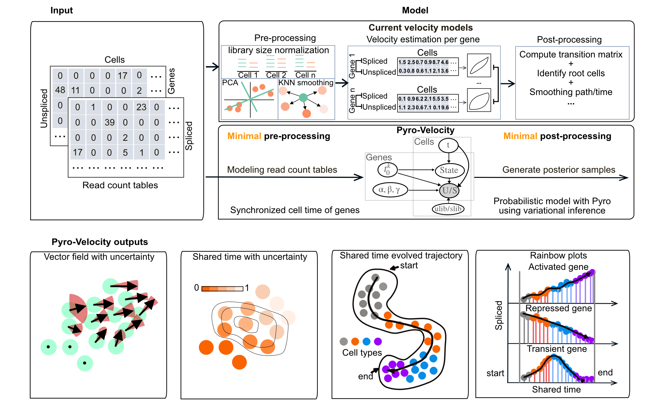
Pyro-Velocity is a Bayesian, generative, and multivariate RNA velocity
model to estimate uncertainty in predictions of future cell states from
minimal models approximating splicing dynamics.
This approach models raw sequencing counts with synchronized cell time across
all expressed genes to provide quantifiable information on
cell fate choice and developmental trajectory dynamics.
Features
- Probabilistic modeling of RNA velocity
- Direct modeling of raw spliced and unspliced read count
- Multiple uncertainty diagnostics analysis and visualizations
- Synchronized cell time estimation across genes
- Multivariate denoised gene expression and velocity prediction
Installation with miniconda
Please install miniconda following the instructions here: https://docs.conda.io/en/latest/miniconda.html, this step takes about 1-2 mins.
wget -c https://repo.anaconda.com/miniconda/Miniconda3-latest-Linux-x86_64.sh
bash Miniconda3-latest-Linux-x86_64.sh
# then follow the instruction to setup the conda base environment
After the conda has been setup, logout and re-login to install mamba to speed up installation, this step takes about 20s.
conda install -c conda-forge mamba
Then add the channels, this step takes 1~2s.
conda config --add channels defaults
conda config --add channels bioconda
conda config --add channels conda-forge
conda config --set channel_priority flexible
After that, install the pyrovelocity package in one mamba command:
mamba create -n pyrovelocity_bioconda -c bioconda pyrovelocity
This step takes about 6-8 minutes depending on the network speed. If you prefer to use conda environment configurations, see the conda subfolder for installation with prefix to specify the installation path, such as:
# GPU
mamba env create --prefix /path_to_conda_env/qq-pyrovelocity-dev -f conda/environment-gpu.yml
# or CPU
mamba env create --prefix /path_to_conda_env/qq-pyrovelocity-dev -f conda/environment-cpu.yml
Or with more control of installing the environment,
conda create -n pyrovelocity_bioconda python=3.8.8
mamba install -n pyrovelocity_bioconda -c bioconda pyrovelocity
# CPU
mamba env update -n pyrovelocity_bioconda -f conda/environment-cpu.yml
# or GPU
mamba env update -n pyrovelocity_bioconda -f conda/environment-gpu.yml
For windows user installation, please refer to the issue.
Lastly, test the installation by:
conda activate pyrovelocity_bioconda
python
import pyrovelocity
Additional packages necessary to reproduce all the analyses presented in the notebooks
pip install cospar==0.1.9
Quick start
After the installation, let's look at your dataset to see how Pyro-Velocity can help understand cell dynamics.
Starting from raw sequencing FASTQ files, obtained for example with SMART-seq, 10X genomics, inDrop or other similar single-cell assays, you can preprocess the data to generate spliced and unspliced gene count tables in h5ad file (or loom file using cellranger+velocyto or the kallisto pipeline.
Starting from these count tables we show below a minimal step-by-step workflow to illustrate the main features of Pyro-Velocity in a Jupyter Notebook:
Step 0. Even though pyrovelocity is a cluster-free method to evaluate uncertainty of cell fate, it will dependend on 2 dimensional embedding results for evaluation of uncertainty and generate visualization, we would suggest run your new datasets using scanpy tutorial.
Step 1. Load your data, load your data(e.g. local_file.h5ad) with scvelo by using:
import scvelo as scv
adata = scv.read("local_file.h5ad")
Step 2. Minimally preprocess your adata object:
adata.layers['raw_spliced']   = adata.layers['spliced']
adata.layers['raw_unspliced'] = adata.layers['unspliced']
adata.obs['u_lib_size_raw'] = adata.layers['raw_unspliced'].toarray().sum(-1)
adata.obs['s_lib_size_raw'] = adata.layers['raw_spliced'].toarray().sum(-1)
scv.pp.filter_and_normalize(adata, min_shared_counts=30, n_top_genes=2000)
scv.pp.moments(adata, n_pcs=30, n_neighbors=30)
Step 3. Train the Pyro-Velocity model:
from pyrovelocity.api import train_model
# Model 1
num_epochs = 1000 # large data
# num_epochs = 4000 # small data
adata_model_pos = train_model(adata,
                               max_epochs=num_epochs, svi_train=True, log_every=100,
                               patient_init=45,
                               batch_size=4000, use_gpu=0, cell_state='state_info',
                               include_prior=True,
                               offset=False,
                               library_size=True,
                               patient_improve=1e-3,
                               model_type='auto',
                               guide_type='auto_t0_constraint',
                               train_size=1.0)

# Or Model 2
adata_model_pos = train_model(adata,
                               max_epochs=num_epochs, svi_train=True, log_every=100,
                               patient_init=45,
                               batch_size=4000, use_gpu=0, cell_state='state_info',
                               include_prior=True,
                               offset=True,
                               library_size=True,
                               patient_improve=1e-3,
                               model_type='auto',
                               guide_type='auto',
                               train_size=1.0)

# adata_model_pos is a returned list in which 0th element is the trained model,
# the 1st element is the posterior samples of all random variables
save_res = True
if save_res:
    adata_model_pos[0].save('saved_model', overwrite=True)
    result_dict = {"adata_model_pos": adata_model_pos[1],
                   "v_map_all": v_map_all,
                   "embeds_radian": embeds_radian, "fdri": fdri, "embed_mean": embed_mean}
    import pickle
    with open("model_posterior_samples.pkl", "wb") as f:
         pickle.dump(result_dict, f)
Step 4: Generate Pyro-Velocity's vector field and shared time plots with uncertainty estimation.
from pyrovelocity.plot import plot_state_uncertainty
from pyrovelocity.plot import plot_posterior_time, plot_gene_ranking,\
      vector_field_uncertainty, plot_vector_field_uncertain,\
      plot_mean_vector_field, project_grid_points,rainbowplot,denoised_umap,\
      us_rainbowplot, plot_arrow_examples

embedding = 'emb' # change to umap or tsne based on your embedding method

# This generates the posterior samples of all vector fields
# and statistical testing results from Rayleigh test
v_map_all, embeds_radian, fdri = vector_field_uncertainty(adata, adata_model_pos[1],
                                                          basis=embedding, denoised=False, n_jobs=30)
fig, ax = plt.subplots()
# This returns the posterior mean of the vector field
embed_mean = plot_mean_vector_field(adata_model_pos[1], adata, ax=ax, n_jobs=30, basis=embedding)
# This plot single-cell level vector field uncertainty
# and averaged cell vector field uncertainty on the grid points
# based on angular standard deviation
fig, ax = plt.subplots(1, 2)
fig.set_size_inches(11.5, 5)
plot_vector_field_uncertain(adata, embed_mean, embeds_radian,
                            ax=ax,
                            fig=fig, cbar=False, basis=embedding, scale=None)

# This generates shared time uncertainty plot with contour lines
fig, ax = plt.subplots(1, 3)
fig.set_size_inches(12, 2.8)
adata.obs['shared_time_uncertain'] = adata_model_pos[1]['cell_time'].std(0).flatten()
ax_cb = scv.pl.scatter(adata, c='shared_time_uncertain', ax=ax[0], show=False, cmap='inferno', fontsize=7, s=20, colorbar=True, basis=embedding)
select = adata.obs['shared_time_uncertain'] > np.quantile(adata.obs['shared_time_uncertain'], 0.9)
sns.kdeplot(adata.obsm[f'X_{embedding}'][:, 0][select],
            adata.obsm[f'X_{embedding}'][:, 1][select],
            ax=ax[0], levels=3, fill=False)

# This generates vector field uncertainty based on Rayleigh test.
adata.obs.loc[:, 'vector_field_rayleigh_test'] = fdri
im = ax[1].scatter(adata.obsm[f'X_{basis}'][:, 0],
                   adata.obsm[f'X_{basis}'][:, 1], s=3, alpha=0.9,
                   c=adata.obs['vector_field_rayleigh_test'], cmap='inferno_r',
                   linewidth=0)
set_colorbar(im, ax[1], labelsize=5, fig=fig, position='right')
select = adata.obs['vector_field_rayleigh_test'] > np.quantile(adata.obs['vector_field_rayleigh_test'], 0.95)
sns.kdeplot(adata.obsm[f'X_{embedding}'][:, 0][select],
            adata.obsm[f'X_{embedding}'][:, 1][select], ax=ax[1], levels=3, fill=False)
ax[1].axis('off')
ax[1].set_title("vector field\nrayleigh test\nfdr<0.05: %s%%" % (round((fdri < 0.05).sum()/fdri.shape[0], 2)*100), fontsize=7)
Step 5: Prioritize putative cell fate marker genes based on negative mean absolute errors and pearson correlation between denoised spliced expression and posterior mean shared time, and then visualize the top one with rainbow plots
fig = plt.figure(figsize=(7.07, 4.5))
subfig = fig.subfigures(1, 2, wspace=0.0, hspace=0, width_ratios=[1.6, 4])
ax = fig.subplots(1)
# This generates the selected cell fate markers and output in DataFrame
volcano_data, _ = plot_gene_ranking([adata_model_pos[1]], [adata], ax=ax,
                                     time_correlation_with='st', assemble=True)
# This generates the rainbow plots for the selected markers.
_ = rainbowplot(volcano_data, adata, adata_model_pos[1],
                subfig[1], data=['st', 'ut'], num_genes=4)
Illustrative examples of Pyro-Velocity analyses on different single-cell datasets
Pyro-Velocity applied to a PBMC dataset [1]
This is a scRNA-seq dataset of fully mature peripheral blood mononuclear cells (PBMC) generated using the 10X genomics kit and containing 65,877 cells with 11 fully differentiated immune cell types. This dataset doesn't contain stem and progenitor cells or other signature of and undergoing dynamical differentiation, thus no consistent velocity flow should be detected.
Below we show the main output generated by Pyro-Velocity Model 1 analysis. Pyro-Velocity failed to detect high-confidence trajectories in the mature blood cell states, consistent with what is known about the biology underlying these cells.
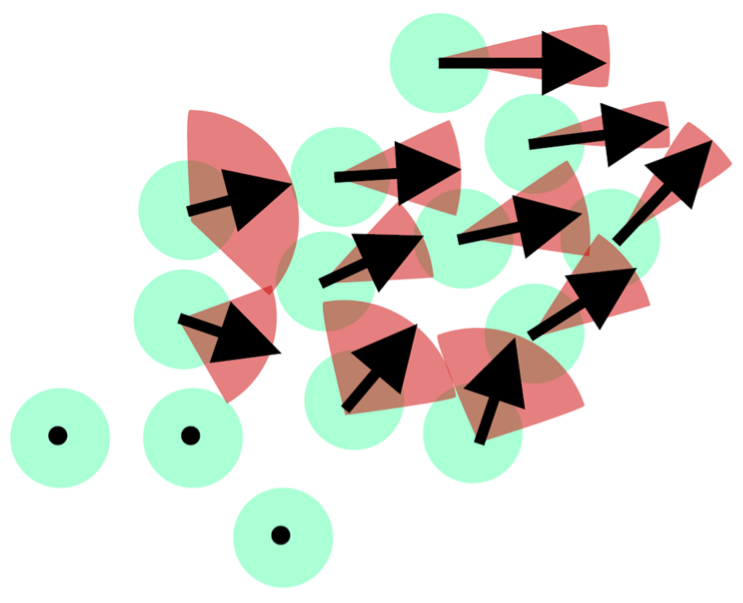
Vector field with uncertainty
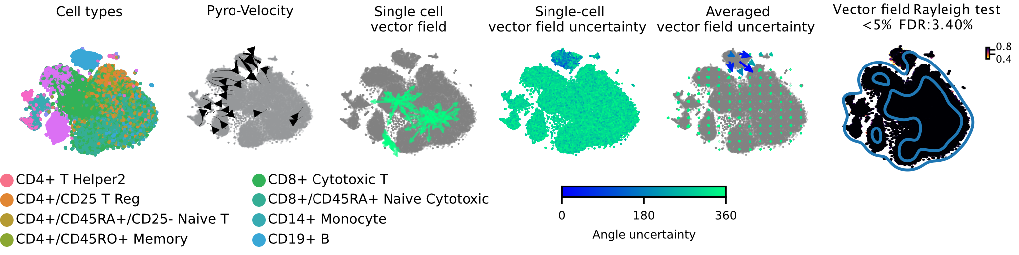
These 6 plots from left to right show: 1. cell types, 2. stream plot of Pyro-velocity vector field based on the posterior mean of 30 posterior samples, 3. single cell vector field examples showing all 30 posterior samples as vectors for 3 arbitrarily selected cells; 4. single cell vector field with uncertainty based on angular standard deviation across 30 posterior samples, 5. averaged vector field uncertainty from 4. 6. Rayleigh test of posterior samples vector field, the title shows the expected false discovery rate using a 5% threshold.
The full example can be reproduced using the PBMC Jupyter notebook.
Pyro-Velocity applied to a pancreas development dataset [2]
Here we apply Pyro-Velocity to a single cell RNA-seq dataset of mouse pancreas in the E15.5 embryo developmental stage. This dataset was generated using the 10X genomics kit and contains 3,696 cells with 8 cell types including progenitor cells, intermediate and terminal cell states.
Below we show the main output generated by Pyro-Velocity Model 1 analysis. Pyro-Velocity was able to define well-known developmental cell hierarchies identifying cell trajectories originating from ductal progenitor cells and culminated in the production of mature Alpha, Beta, Delta, and Epsilon cells.
Vector field with uncertainty
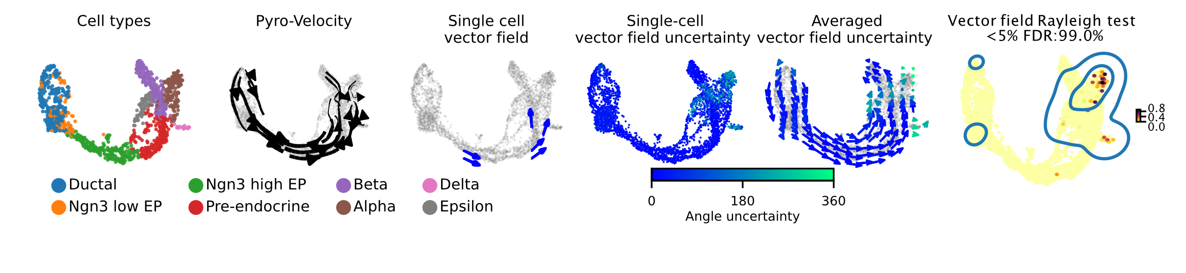
These 6 plots from left to right are showing the same analyses presented as in the example above.
Shared time with uncertainty
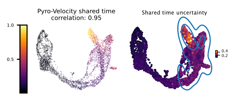
The left figure shows the average of 30 posterior samples for the cell shared time, the title of the figure shows the Spearman's correlation with the Cytotrace score, an orthogonal state-of-the-art method used to predict cell differentiation based on the number of expressed genes per cell (Gulati et. al, Science 2020). The right figure shows the standard deviation across posterior samples of shared time.
Gene selection and visualization
To uncover potential cell fate determinant markers genes of the mouse pancreas, we first select the top 300 genes with the best velocity model fit (we use negative mean absolute error ), then we rank the filtered genes using Pearson's correlation between denoised spliced expression and the posterior mean of the recovered shared time across cells.
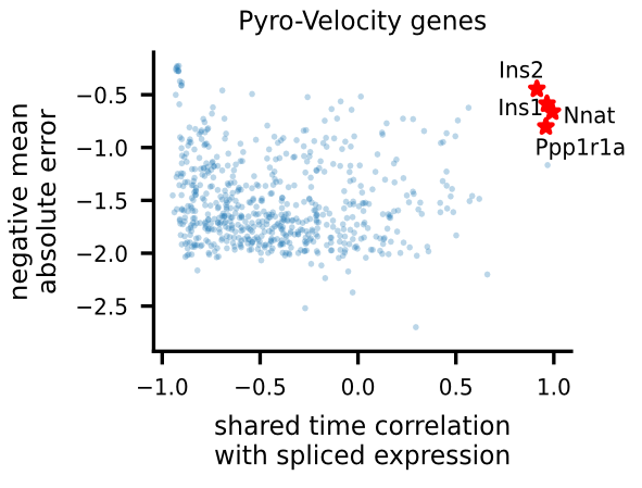
For the selected genes, it is possible to explore in depth their dynamic, using phase portraits, rainbow plots, and UMAP rendering of denoised splicing gene expression across cells.
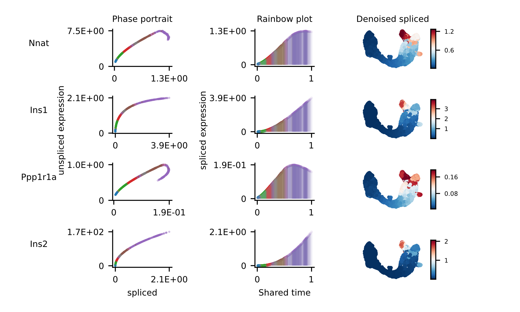
The full example can be reproduced using the Pancreas jupyter notebook.
Pyro-Velocity applied to the LARRY dataset [3]
This last example, present the analysis of a recent scRNA-seq dataset profiling mouse hematopoises at high resolution thanks to lineage relationship information captured by the Lineage And RNA RecoverY (LARRY) system. LARRY leverages unique lentiviral barcodes that enables to clonally trace cell fates over time (Weinrab et al. Cell 20).
Below we show the main output generated by Pyro-Velocity analysis.
Vector field with uncertainty
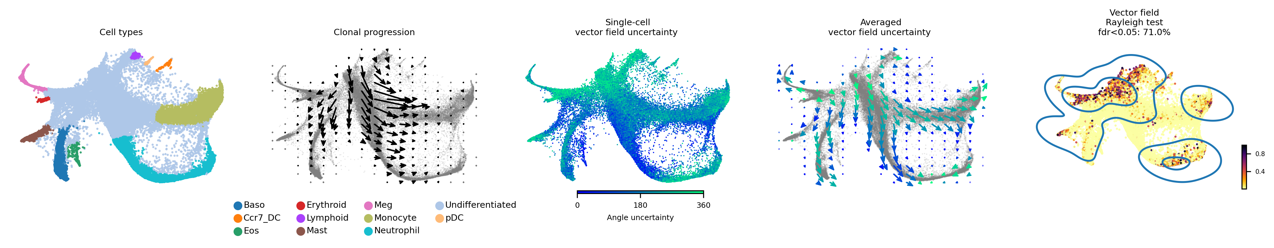
These 5 plots from left to right shows: 1) Cell types, 2) Clone progression vector field by using centroid of cells belonging to the same barcode for generating directed connection between consecutive physical times, 3) single cell vector field with uncertainty based on angular standard deviation across 30 posterior samples, 4. averaged vector field uncertainty from 3. 5. Rayleigh test of posterior samples vector field, the title shows the false discovery rate using threshold 5%.
Shared time with uncertainty
To quantitatively assess the quality of the the receovered shared time we also considered the agreement of our method with Cospar, a state-of-the-art method specifically designed for predicting fate potency based on LARRY data.
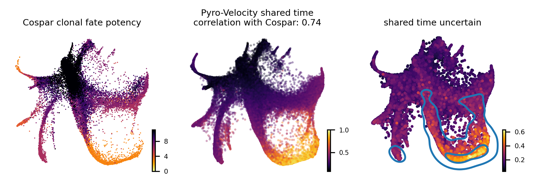
The leftmost figure shows the Cospar fate potency score, the middle figure shows the average of 30 posterior samples from Pyro-Velocity shared time per cell, the title of the figure shows the Spearman's correlation between cell latent shared time and fate potency scores derived from Cospar, the right figure shows the standard deviation across posterior samples of shared time.
The full example can be reproduced using the LARRY jupyter notebook.
Troubleshooting
TypeError: fate_potency() got an unexpected keyword argument 'used_Tmap'
Please use the specific cospar version:
pip install cospar==0.1.9
CUDA error: no kernel image is available for execution on the device
All reference to GPU support applies to linux. We do not currently support windows
and there is no GPU-compatible pytorch version <1.12 for darwin.
On linux, either use conda (as exemplified in
reproducibility/environment),
or install the specific cuda-enabled pytorch version manually
pip3 install torch==1.8.1+cu111 -f https://download.pytorch.org/whl/torch_stable.html
If you are using poetry, you can also use the poetry helper
poetry install && poetry run poe force-cuda11
Also see contributing.
Release history Release notifications | RSS feed


Download files
Download the file for your platform. If you're not sure which to choose, learn more about installing packages.
Source Distribution
Built Distribution
Hashes for pyrovelocity-0.1.1-py3-none-any.whl
| Algorithm | Hash digest | |
|---|---|---|
| SHA256 | ce916bd116c9664919f4b6887158d1a0c0c7f5a43f5759fe8204a0f6eb09aad1 |
|
| MD5 | e179a9c67f4390ec69d2dd7fe2360704 |
|
| BLAKE2b-256 | 836ea8ac2d359fd7075241529c363b58ff5af3fc806c6c655a198e5669edf833 |


