A differential equation solver using quantum annealing. It can be applied to coupled linear ODEs and PDEs with variable coefficients and inhomogeneous terms. The solution is obtained by finding the optimal weights for a linear combination of "basis functions":

The problem can then be viewed as a minimization one, for the loss function

where E is the equation to be solved, B are the initial/boundary conditions, and the x are the sample points at which they must hold. From this perspective, there is no difference between the equation and the boundary conditions, and they are treated on an equal footing. The loss function is then translated into an Ising model Hamiltonian by means of a binary encoding for the weights and solved in a quantum annealer.

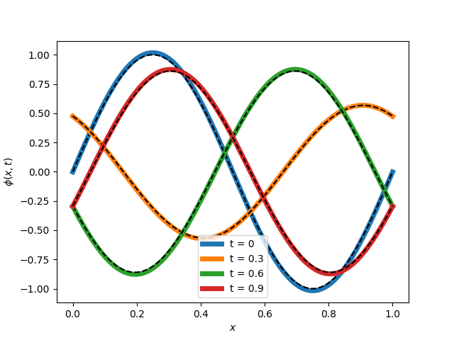
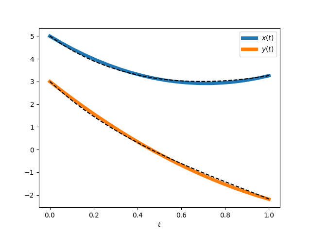
Solutions obtained with qade for the wave equation and a system of coupled first order ODEs (see the examples directory):

Contents

• Installation
• Usage example
• Documentation
  • qade.function
  • qade.basis
  • qade.equation
  • qade.solve
  • Inspecting the loss function
• Citation

Installation

> pip install qade

This will install the dependencies numpy and dwave-ocean-sdk if not present. Python version 3.7 or higher is required. In order for qade to send the problem for solution in the D-Wave systems, the API token needs to be configured.

Usage example

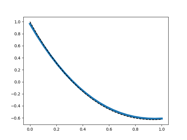
As an example, we can solve the Laguerre equation in the [0, 1] interval with boundary conditions at the extremes:

where L_n is the nth Laguerre polynomial. To do so, we parametrize the solution as a linear combination of the first few powers of x, and look for the optimal values of the weights such that the equation is satisfied at a set of sample points. This can be done through:

import numpy as np
from scipy.special import eval_laguerre as L
import qade

n = 4  # Laguerre equation parameter
x = np.linspace(0, 1, 20)  # Sample points at which the equation is to be evaluated
y = qade.function(n_in=1, n_out=1)  # Define the function to be solved for

# Define the equation and boundary conditions
eq = qade.equation(x * y[2] + (1 - x) * y[1] + n * y[0], x)
bcs = qade.equation(y[0] - [1, L(n, 1)], [0, 1])

# Solve the equation using as the basis of functions the monomials [1, x, x^2, x^3]
y_sol = qade.solve([eq, bcs], qade.basis("monomial", 4), scales=(n - 2), num_reads=500)

This illustrates the use of the 4 main functions provided by qade:

• qade.function(n_in, n_out) defines a symbolic function y of n_in inputs and n_out outputs, whose nth derivative is denoted as y[n].

• qade.equation(eq, samples) defines an equation of the form eq == 0, with samples being an array-like object containing sample points at which it holds.

• qade.basis(name, size_per_dim, ...) defines the basis of functions in terms of which the solution will be written.

• qade.solve(eqs, basis, ...) uses a binary encoding to represent the problem of solving the given equations in the given basis as an Ising model, sends it to a D-Wave quantum annealer, and collects it into a Solution object y_sol.

We can now print the weights of the basis functions in the solution and the corresponding through:

print(f"loss = {y_sol.loss:.3}, weights = {y_sol.weights}")

We can also evaluate the solution at any set of points, plot the results, and compare to the analyical solution, the which is nth Laguerre polynomial:

import matplotlib.pyplot as plt

plt.plot(x, y_sol(x), linewidth=5)
plt.plot(x, L(n, x), color="black", linestyle="dashed")
plt.show()

For other examples, see the examples directory. An example PDE, the wave equation, is solved in wave.py. A system of coupled first-order ODEs is solved in coupled.py.

Documentation

qade.function

Creates Function objects, to be used in definition of the equations. The arguments are:

• n_in: int. The number of input variables of the function, i.e. the dimension of the domain.

• n_out: int. The number of output variables of the function, i.e. the dimension of the target space. For n_out == 1, qade.function returns a single Function. For n_out > 1, it returns list of Function objects, one for each output component.

A differential equation or boundary condition is then defined as a linear combination of the derivatives of the functions, plus possible an inhomogeneous term, with coefficients and inhomogeneous term being either scalars or flat array-like objects (numpy arrays, lists, ...) having the same length as the set of sample points at which the equation is evaluated. The examples show how this is done in different practical settings. The notation f[k1, ..., kn] represents the following expression:

qade.equation

Creates an Equation, representing any linear differential equation or boundary condition. The arguments are:

• formula. The expression for the equation, constructed as a linear combination of derivatives f[k1, ..., kn] of Function objects, plus the optional inhomogeneous term.

• samples, an array-like object of shape (n_samples, n_in) (or just (n_samples,), if n_in == 1). Defines the sample points from the domain in which the equation must hold.

qade.basis

Creates a Basis, representing the functions to be linearly combined into the solution. The arguments are:

• name: str. The allowed names are:

  • "fourier". A product of the following functions for each component x in the input space:

    

  • "monomial". A product of the following functions for each component x in the input space:

    

  • "trig". A product of the following functions for each component x in the input space:

    

  • "gaussian". The following functions of the distance r to each point x_n in an equally-spaced grid in the input space (which is assumed to be the box [0, 1]^n_in):

    

  • "multiquadric". The following functions of the distance r to each point x_n in an equally-spaced grid in the input space (which is assumed to be the box [0, 1]^n_in):

    

• size_per_dim: int. The number of functions to use per input variable. The total dimension of the basis will be size_per_dim ** n_in.

• n_in: int. Only used by the radial basis functions "gaussian" and "multiquadric" to create the grid of points in the domain.

• scale: float. The lambda scale parameter of the radial basis functions "gaussian" and "multiquadric".

Custom bases

Custom bases can be provided by the user. In this case, instead of using qade.basis, the user should define a class implementing the methods:

• dimension(self, n_in: int) -> int. Returning the total number of functions in the basis.

• derivatives(self, k: int, samples: np.ndarray) -> np.ndarray. Returning the array of kth derivatives of the basis functions at the given sample points, received as an array of shape (n_samples, n_in). The output array should have shape: (n_samples, n_out) + (n_in,) * k.

qade.solve

Solves the given equations and returns a Solution object. The arguments are:

• equations: List[Equation]. The equations to be solved, including initial/boundary conditions.

• basis: Basis. The basis to be used in their solution.

• n_spins: int = 3. The number of spins per weight in the binary encoding.

• n_epochs: int = 10. The number of epochs in which the problem is solved, using the values obtained in the previous epoch as the center values in the binary encoding of the weights.

• scale_factor: float = 0.5. The relative change in the scale in the binary encoding of the weights from one epoch to the next.

• anneal_schedule: Optional[List[Tuple[int, int]]] = None. The schedule to be used by the quantum annealer. See D-Wave Ocean Tools' documentation for details. If None, it will default to a linear schedule of the form [(0, 0), (200, 0)].

• num_reads: int = 200. The number of reads to be performed by the quantum annealer.

• qpu_solver: str = "Advantage_system4.1". The QPU to be used.

• centers: ArrayLike = 0. The initial central values in the binary encoding of the weights. Must be a scalar or an array of size n_out * basis_dim.

• scales: ArrayLike = 1. The initial scales in the binary encoding of the weights. Must be a scalar or an array of size n_out * basis_dim.

• verbose: bool = False. Determines if information about intermediate steps should be printed.

• classical_minimizer: Optional[Callable[[Callable[[np.ndarray], float]], np.ndarray]] = None. If not None, a classical function to be used in place of the quantum procedure for minimizing the loss function, for testing purposes.

Solution objects

Return type of qade.solve. They are callables that receive an array-like object of sample points, with shape (n_samples, n_in) (or just (n_samples,), if n_in == 1), and return the corresponding values of the solution, as a numpy array of shape (n_samples, n_out). Their attributes are:

• basis: Basis. The basis in terms of which the solution has been obtained.

• weights: np.ndarray, with shape (n_out, n_in). The optimal weights providing the solution as a linear combination of the basis functions.

• loss: float. The value of the loss function at the given weights.

Inspecting the loss function

Two functions are provided to obtain the internal parameters of the loss function, both as a quadratic function of the real-valued weights, and as an Ising model Hamiltonian in the annealer spins.

qade.loss

Returns the (J, h) parameters of the quadratic loss function Q(w) = w^T J w + h^T w, where w is the flattened array of the continuous weights. The arguments are

• equations: List[Equation]. The equations to be included.

• basis: Basis. The basis to be used in their solution.

qade.ising

Returns the (J, h) parameters of the Ising model Hamiltonian H(w) = w^T J w + h^T w, where w is the flattened array of spins. The arguments are:

• equations: List[Equation]. The equations to be included.

• basis: Basis. The basis to be used in their solution.

• n_spins: int = 3. The number of spins per weight in the binary encoding.

• centers: ArrayLike = 0. The initial central values in the binary encoding of the weights. Must be a scalar or an array of size n_out * basis_dim.

• scales: ArrayLike = 1. The initial scales in the binary encoding of the weights. Must be a scalar or an array of size n_out * basis_dim.

Citation

If you use qade, please cite: