Small utility for fetching, and manipulating Sea Level Rise Projections from various sources for engineering calculations

Project description
Python Sea Level Rise (sealevelrise)
sealevelrise is simple Python package designed to aggregate, load, and display sea level rise projectsion from multiple sources.
What SLR Does
sealevelrise provides convenient classes and methods to perform routine tasks most commmonly
encountered by practicioners in the civil industry:
- Load sea-level rise projections for a specific location using builtin scenarios or from or a variety of APIs and methods
- Display trajectories over time as plots or tables
- Evaluate sea-level rise offset by a certain horizon date
- Compare risk-based sea-level rise trajectories
- Compare historical and future trajectories
- Convert units and modify reference water levels
- Combine projections with historical trends retrieved from NOAA API
Basic Structure
SLR relies on three classes to organize SLR data:
SLRProjectionscontains a collection ofScenarioitems for a given location (e.g., a city or a state)ScenariocontainsDatadescribing a specific SLR trajectoryDatacontains the timeline, units, and values for that SLR trajectory
The class hierarchy is illustrated in the Class Diagram, below.
classDiagram
    class Data
    Data : +np.array x
    Data : +np.array y
    Data : +str units
    Data : +convert()

    class Scenario
    Scenario : +string description
    Scenario : +string short_name
    Scenario : +float baseline_year
    Scenario : +Data data
    Scenario : +str units
    Scenario : +dataframe() DataFrame
    Scenario : +by_horizon_year() float

    class SLRProjections
    SLRProjections : +tuple shape
    SLRProjections : +str location_name
    SLRProjections : +scenarios [Scenario]
    SLRProjections : +str station_ID
    SLRProjections : +str issuer
    SLRProjections : +pd.DataFrame dataframe
    SLRProjections : +from_location() SLRProjections
    SLRProjections : +show_all_available_locations() list
    SLRProjections : +by_horizon_year() array
    SLRProjections : +convert() array
    SLRProjections : +plot() Axes


    Data "1" --* "1" Scenario
    Scenario "*" --* "1" SLRProjections
Builtin Scenarios and Online Sources
Scenarios can be loaded from a variety of sources including:
- use one of the many builtin scenarios (see under
\data\scenarios.json) - invoke NOAA API for the latest set of projections
Extensibility
Add your own custom builtin scenarios by modifying and contributing to the scenarios.json file.
Installation
The preferred way is to pip install directly from GitHub.com into a virtual environment:
>>> python -m pip install <absolute_cloned_repo_root_directory>
Quickstart (Jupyter)
SLR provides a very easy way to manipulate sea-level rise scenario datasets. The SLR package was built with convenience in mind and is designed to facilite operations commonly encountered when dealing with sea-level rise projections at specific locations. It is primarily designed to be used within Jupyter and is geared toward practitioners who need to publish their findings in reports.
Importing SLR
Assuming you installed the package or appended to PYTHONPATH, all that remains to do is to import the package:
>>> import sealevelrise
Show All Builtin Scenarios
From that point on, we can list all locations available in the scenarios.json file: these are as many SLRProjections items:
>>> sealevelrise.SLRProjections.show_all_builtin_scenarios(format='list')
The locations can be displayed as a pandas.Dataframe for further manipulation:
>>> sealevelrise.SLRProjections.show_all_builtin_scenarios(format='dataframe')
Manipulating SLR Scenarios
Let's load a SLRProjections by invoking a builtin location:
>>> sf = sealevelrise.SLRProjections.from_location_or_key(
    location_or_key="San Francisco, CA"
)
We could do the same using index notation:
>>> sf = sealevelrise.SLRProjections.from_index(index=1)
Or we could do the same thing using a key from the scenarios.json file:
>>> sf = sealevelrise.SLRProjections.from_key(key="cocat-2018-9414290")
All the SLR projections contained within the SLRProjections can be displayed in iPython and copy/pasted into a report
>>> sf.dataframe
Converting Units
In some cases, units may need to be converted. SLR offers on-the-fly capabilities for converting Data to any of the allowable units. For example:
>>> sf.convert(to_units='in')
The conversion takes place in-place. On-the-fly conversion is not (yet) supported.
Visualization
We can plot Scenario items within a SLRProjections right away: all Scenario items are
plotted automatically by default.
>>> sf.plot()
We can also combine commands. In this case, let's convert to feet for easier interpretation and let's add a target date to show on the plot.
>>> sf.convert(to_units='ft')
>>> sf.plot(horizon_year=2075)
>>> plt.tight_layout()
Here is what this should look like:
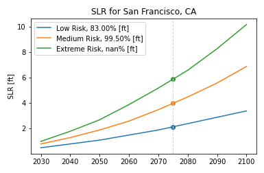
By default, all Scenario items within a given SLRProjections will be plotted.
To select specific Scenario items see Section Drilling Into Specific Scenarios below.
Calculating Projections by a Certain Date
We can calculate the effective SLR projections by a certain date, e.g.:
sf.by_horizon_year(2075, merge=False)
We can also choose to merge that projection into the resultant dataframe, for presentation purposes. Note that the SLRProjections item is not affected by the merging operation, it is only for displaying purposes.
sf.by_horizon_year(horizon_year=2075, merge=True)
Drilling Into Specific Scenarios
Each SLRProjections item contains one or more Scenario items which can be conveniently retrieved using index notation:
sf_scenario = sf[1]
sf_scenario
And here is what it should look like:
Scenario 'Medium Risk', values are given in in and years range from 2030 to 2100
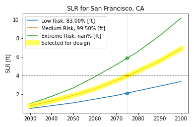
This allows to "drill down" into the scenarios. Let's return to our prior example of visualization, and let's manipulate a specific scenario:
# Display a base figure using the builtin method
ax = sf.plot(horizon_year=2075)
# Highlight the specific Scenario item retained for design
ax.plot(sf_scenario.data.x, sf_scenario.data.y, c='yellow', label='Selected for design', lw=10, alpha=.65)
# Use the builtin class method to estimate SLR by the horizon year
ax.axhline(y=sf_scenario.by_horizon_year(horizon_year=2075), c='k', ls='--', lw=1)
# Update the legend
plt.legend()
plt.tight_layout()
Here is what this should now look like:
Comparing with the Historical Rate New
You can attempt to retrieve the historical sea-level rise from NOAA servers. To do that, simply create a new HistoricalSLR instance:
>>> HistoricalSLR.from_station(id=<your_NOAA_station_ID>)
Customizing the scenarios.json File
SLR works by loading a JSON file located under .\data\scenarios.json. The format of the file mimics the structure of SLRProjections, Scenario, and Data class items. An example is shown for San Francisco, CA. The data was extracted from the 2018 State of California Sea-level Rise Guidance document published by the Ocean Council. SLR is built upon that publication but can be used to handle other guidelines, as long as the same nomenclature is used.
Basic Structure
The structure of the JSON file mimics the classes used in SLR. An extract of the file is shown below:
{
    "San Francisco": {
        "description": "San Francisco, CA",
        "station ID (CO-OPS)": "9414290",
        "scenarios": [
            {
                "description": "High Emission, Low Risk (Likely Range)",
                "short name": "Low Risk",
                "units": "ft",
                "probability (CDF)": 0.83,
                "baseline year": 2000,
                "data": {
                    "x": [
                        2030,
                        2040,
                        2050,
                        2060,
                        2070,
                        2080,
                        2090,
                        2100
                    ],
                    "y": [
                        0.5,
                        0.8,
                        1.1,
                        1.5,
                        1.9,
                        2.4,
                        2.9,
                        3.4
                    ]
                }
            },
            {
                "description": "High Emission, Medium-High Risk (1-in-200 Chance)",
                "short name": "Medium Risk",
                "units": "ft",
                "probability (CDF)": 0.995,
                "baseline year": 2000,
                "data": {
                    "x": [
                        2030,
                        2040,
                        2050,
                        2060,
                        2070,
                        2080,
                        2090,
                        2100
                    ],
                    "y": [
                        0.8,
                        1.3,
                        1.9,
                        2.6,
                        3.5,
                        4.5,
                        5.6,
                        6.9
                    ]
                }
            },
            {
                "description": "High Emission, Extreme Risk (H++ Scenario)",
                "short name": "Extreme Risk",
                "units": "ft",
                "probability (CDF)": null,
                "baseline year": 2000,
                "data": {
                    "x": [
                        2030,
                        2040,
                        2050,
                        2060,
                        2070,
                        2080,
                        2090,
                        2100
                    ],
                    "y": [
                        1.0,
                        1.8,
                        2.7,
                        3.9,
                        5.2,
                        6.6,
                        8.3,
                        10.2
                    ]
                }
            }
        ]
    }
}
Adding New Locations and Projections
New locations can be added using the same nomenclature. Currently, the following fields are implemented:
- "ID": a unique key for each
SLRProjectionsitem- "location name": the location for these SLR scenarios, e.g., "San Francisco, CA"; a unique location defines a given
SLRProjections - "station ID (CO-OPS)": the NOAA or CO-OPS identification string for the location, if available, e.g, "9414290", a unique location defines a given
SLRProjections - "scenarios": an array of JSON items containing specific
Scenarioitems
- "location name": the location for these SLR scenarios, e.g., "San Francisco, CA"; a unique location defines a given
Each Scenario item consists of the following:
- description: describes the
Scenario, e.g. "Extreme High" - short name: a short description of the Scenario, used in plots for example
- units: can only be one of the allowable values (see below section)
- probability: a number specifying the probability (CDF) of the
Scenario, 0 to 1. - baseline year: the value for the baseline year for the
Scenario - data: dict, a dictionary representing the
Dataitem, itself comprising two elements:- "x" : an array containing the years where projections are provided
- "y" : an array containing the values for sea-level rise at these years, in the units referenced above
Allowable Units
Supported units are limited to the following:
- 'ft' : feet (US)
- 'm' : meters
- 'cm' : centimeters
- 'in' : inches
Release history Release notifications | RSS feed


Download files
Download the file for your platform. If you're not sure which to choose, learn more about installing packages.
Source Distribution
Built Distribution
Hashes for sealevelrise-0.1.1-py3-none-any.whl
| Algorithm | Hash digest | |
|---|---|---|
| SHA256 | 05fdc515c12bac0304b6fe07e9e0fa0933f2b5a2c2e65e5b978dc2f4dc306cb3 |
|
| MD5 | fe3a727744a8dabefb262bc67e85f8b7 |
|
| BLAKE2b-256 | 4c6cafee24eada678cd4b67eca2fcd140667dfbe29aad382f93d1802f4af0b7b |


