Shape DTW python package

shapedtw-python is an extension to the dtw-python package, implementing the shape dtw algorithm described by L. Itii and J. Zhao in their paper (it can be downloaded from here: shapeDTW: shape Dynamic Time Warping).

In addition, to enable users to fully exploit the potential of the dtw and shape-dtw algorithms in practical applications, we have enabled the use of both versions of the multidimensional variant of the algorithm (dependent and independent), according to the methodology described in the paper by B. Hu, H. Jin, W. Keogh, M. Shokoohi-Yekta and J. Wang: Generalizing DTW to the multi-dimensional case requires an adaptive approach.

Github repository of the shapedtw-python project can be found here: shapedtw-python.

Introduction to the shape dtw algorithm

In order to fully understand the shape dtw algorithm it is good to know the methods for calculating standard dtw. We recommend to get familiarized with classic work of S. Chiba and H. Sakoe (available online here: Dynamic Programming Algorithm Optimization for Spoken Word Recognition, however one can prefer to read this shorter, yet comprehensive guide: An introduction to Dynamic Time Warping

Shape descriptors

In case of standard DTW we use raw time series values to determine the alignment (warping) path by which two signals (time series) can be aligned in time. Such alignment may be susceptible to local distortion and therefore does not fully reflect the correct relationships between signals. Zhao and Itti proposed to solve this problem by using so-called shape descriptors, instead of single points of time series:

Yet, matching points based solely on their coordinate values is unreliable and prone to error, therefore, DTW may generate perceptually nonsensible alignments, which wrongly pair points with distinct local structures (...). This partially explains why the nearest neighbor classifier under the DTW distance measure is less interpretable than the shapelet classifier [35]: although DTW does achieve a global minimal score, the alignment process itself takes no local structural information into account, possibly resulting in an alignment with little semantic meaning. In this paper, we propose a novel alignment algorithm, named shape Dynamic Time Warping (shapeDTW), which enhances DTW by incorporating point-wise local structures into the matching process. As a result, we obtain perceptually interpretable alignments: similarly-shaped structures are preferentially matched based on their degree of similarity. (...)

Itti, L.; Zhao, J., shapeDTW: shape Dynamic Time Warping, Pattern Recognition, Volume 74, pp. 171-184, Feb 2018.

According to Zhao and Itti shape descriptor encodes local structural information around the temporal point t_i.

In order to calculate shape descriptor we need to - as a first step - retrieve the subsequences for all points of given time series. Subsequences are simply a subsets of time series, representing neighbourhood of particular temporal observation, which is a central point of given subsequence.

As a next step we need to calculate shape descriptors for all the subsequences. Shape descriptor is simply a function applied to given subsequence, which allows to properly describe its local shape's properties (like slope, mean values, wavelet coefficients, etc.). The most simple shape descriptor might be a raw subsequence itself.

Then, we calculate the distance matrix - required by the dtw algorithm - based on obtained shape descriptors instead of raw, single values of time series. Finally warping path is determined based on such distance matrix.

Types of shape descriptors

• Raw subsequence - raw subsequence; there is no any transformation applied to it.
• PAA - subsequence is split into m disjoint intervals. For each interval we calculate mean value of temporal points falling into it. Vector of such mean values is our shape descriptor.
• DWT - Discrete Wavelet Transform is applied to whole subsequence. Wavelet coefficients are bound into the form of vector, which we use as a shape descriptor.
• Slope - similarly as in case of PAA we split subsequence into m disjoint intervals and fit a line according to points falling within each interval. Slopes of lines are bound to the form of vector and use as a shape descriptor. This type of shape descriptor is invariant to y-shift.
• Derivative - first order derivatives of given subsequence, calculated using the formula presented in this paper: Derivative Dynamic Time Warping.Similarly as slope descriptor it is invariant to y-shift.
• Compound descriptor - two or more shape descriptors bound into a form of single vector. We can use weights to compensate for differences in average descriptor values.

All shape descriptors listed above are described in details in Zhao and Itti paper.

Code examples

Quick example

Below is a brief example for anyone who wants to get started quickly with the 'shape dtw' algorithm.

Let's calculate shape dtw alignment and distance for two time series, one of which is slightly shifted and distorted with respect to the other.

As a first step we need to make necessary imports:

import numpy as np
import pandas as pd
from numpy.random import randn
from shapedtw.shapedtw import shape_dtw
from shapedtw.shapeDescriptors import SlopeDescriptor, PAADescriptor, CompoundDescriptor
from shapedtw.dtwPlot import dtwPlot

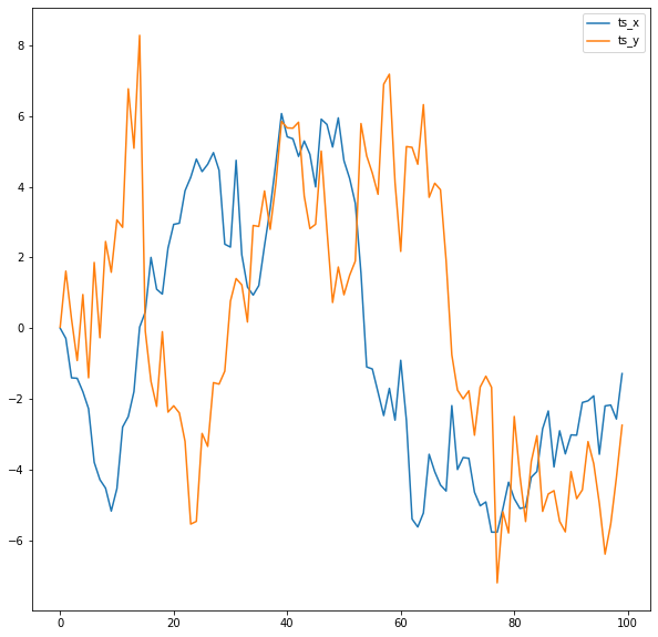
Now let's define input time series and take a look at them:

np.random.seed(9)
distortion_factor = 1
ts_x = np.cumsum(randn(100))
ts_y = np.concatenate(
    (
        np.cumsum(randn(15)),
        ts_x[:85]
    )
) + (randn(100)*distortion_factor)

df = pd.DataFrame({"ts_x": ts_x, "ts_y": ts_y})
df.plot()

As a final step we will define shape descriptor and run the algorithm to obtain alignment path. We will use compound descriptor, consisting of slope descriptor (y-shift invariant) and PAA descriptor.

slope_descriptor = SlopeDescriptor(slope_window=5)
paa_descriptor = PAADescriptor(piecewise_aggregation_window=5)
compound_descriptor = CompoundDescriptor([slope_descriptor, paa_descriptor],descriptors_weights=[5., 1.])
shape_dtw_results = shape_dtw(
    x=ts_x,
    y=ts_y,
    subsequence_width=20,
    shape_descriptor=compound_descriptor
)

dtwPlot(shape_dtw_results, plot_type="twoway", yoffset = 30)

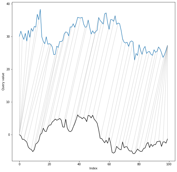
As we can see, despite the shift and distortion of the reference series, the shape dtw algorithm has reproduced the true alignment path almost completely correctly.

Finally, we can retrieve a distances from shape_dtw_results object in the following way:

print(round(shape_dtw_results.distance, 2))
196.58

print(round(shape_dtw_results.normalized_distance, 2))
0.98

print(round(shape_dtw_results.shape_distance, 2))
1276.43

print(round(shape_dtw_results.shape_normalized_distance, 2))
6.38

distance and normalized_distance are distances between raw values of time series, whereas shape_distance and shape_normalized_distance are distances between shape descriptors of time series. Details are explained in the sections below.

Calculation process in details

The whole process of calculating shape dtw consists out of a few steps:

• Transform time series to the matrix of subsequences. In multivariate case each dimension is transformed to individual subsequence's matrix.
• Transform subsequences to shape descriptors using chosen mapping function (shape descriptor).
• Calculate distance matrix between shape descriptors.
• Pass distance matrix to dtw function from dtw-python package in order to calculate warping path and distance.
• Calculate distance for raw time series values using warping path determined by shape dtw.

Although - as we saw in the previous section - shapedtw-python package implements whole pipeline described above in a single call to the shape_dtw function, we will go through all this steps in this document in order to get better understanding of the whole process.

As a first step we will define short, univariate time series and transform them to subsequences. In order to do this we will need to import UnivariateSubsequenceBuilder class from preprocessing module.

import numpy as np
from shapedtw.preprocessing import UnivariateSubsequenceBuilder

subsequence_width = 1

ts_x = np.array([1, 2, 3, 4])
ts_y = np.array([11, 12, 13, 14])


ts_x_subsequences = UnivariateSubsequenceBuilder(
    ts_x, subsequence_width
).transform_time_series_to_subsequences()
ts_y_subsequences = UnivariateSubsequenceBuilder(
    ts_y, subsequence_width
).transform_time_series_to_subsequences()

print(ts_x_subsequences.subsequences)
[[1 1 2]
 [1 2 3]
 [2 3 4]
 [3 4 4]]

print(ts_y_subsequences.subsequences)
[[11 11 12]
 [11 12 13]
 [12 13 14]
 [13 14 14]]

Parameter subsequence_width controls the width of subsequence. For subsequence_width=1 the entire subsequence has a length of 3 (for each temporal point we take one predecessor and one successor). At the beginning and at the end of time series we need to replicate first and last observation in order to make subsequences well-defined for all of temporal points.

Actually, we can consider standard dtw as a special case of shape dtw with subsequence_width=0 and RawSubsequenceDescriptor as a shape descriptor.

As a next step we will calculate shape descriptors for all subsequences using the PAA descriptor.

from shapedtw.shapeDescriptors import PAADescriptor

paa_descriptor = PAADescriptor(piecewise_aggregation_window=2)
ts_x_shape_descriptors = ts_x_subsequences.get_shape_descriptors(paa_descriptor)
ts_y_shape_descriptors = ts_y_subsequences.get_shape_descriptors(paa_descriptor)

print(ts_x_shape_descriptors.shape_descriptors_array)
[[1.  2. ]
 [1.5 3. ]
 [2.5 4. ]
 [3.5 4. ]]

print(ts_y_shape_descriptors.shape_descriptors_array)
[[11.  12. ]
 [11.5 13. ]
 [12.5 14. ]
 [13.5 14. ]]

Windowing descriptors, such as slope or PAA split subsequences into disjoint intervals. In a situation such as above, when it is not possible to divide the sub-sequence into n intervals of equal length, the length of the last interval is equal to the remainder of the division length of the subsequence / length of the window. In this case, the first value of the PAA descriptor is the average value of the first two values of the subsequence, and the second value of the PAA descriptor is the third value of the subsequence.

Finally, the distance matrix between the shape descriptors is calculated and passed to the dtw.dtw function along with other parameters (originally these additional parameters are passed to the shape_dtw function).

from dtw import dtw

distance_matrix = ts_x_shape_descriptors.calc_distance_matrix(ts_y_shape_descriptors)
dtw_results = dtw(distance_matrix.dist_matrix)

print(round(dtw_results.distance, 2))
89.5

print(round(dtw_results.normalizedDistance, 2))
11.19

Please bare in mind that distance calculated in such a way is a distance between shape descriptors of time series, not time series itself. Of course it can be treated as a distance measure and used for example to find nearest neighbour in classification tasks, however one can prefer to use distance between raw values of time series. In order to reconstruct such distance, we can use DistanceReconstructor class.

In case of shape_dtw function raw distances are calculated by defult and available as distance and normalized_distance attributes of classes representing shape dtw results.

To calculate raw distances we must provide raw time series, warping path determined by the shape dtw algorithm, step pattern and distance method which were used. In the example above, we have used the step pattern symmetric2 and euclidean distance, as these are the default values for these parameters.

from shapedtw.shapedtw import DistanceReconstructor

dist_reconstructor = DistanceReconstructor(
    step_pattern="symmetric2",
    ts_x=ts_x,
    ts_y=ts_y,
    ts_x_wp=dtw_results.index1s,
    ts_y_wp=dtw_results.index2s,
    dist_method="euclidean"
)

raw_ts_distance = dist_reconstructor.calc_raw_ts_distance()
print(round(raw_ts_distance, 2))
8.45

Normalized raw distance is calculated internally by class representing shape dtw results, using the step pattern settings.

Multidimensional variants of shape dtw

For multidimensional time series we need to create subsequence matrix and shape descriptor matrix for each dimension separately. There are two variants of multivariate shape dtw - dependent and independent. Differences between those variants are described in details in the paper mentioned above: Generalizing DTW to the multi-dimensional case requires an adaptive approach.

The most important information is that in case of multivariate dependent shape dtw there is one, common warping path for the whole time series. As for independent variant, each dimension has his own warping path, calculated independently for it. We can select desired variant specifying multivariate_version parameter of shape_dtw function as 'dependent' or 'independent':

import numpy as np
from numpy.random import randn
from shapedtw.shapedtw import shape_dtw
from shapedtw.dtwPlot import dtwPlot
from shapedtw.shapeDescriptors import SlopeDescriptor

np.random.seed(9)
ts_x = np.cumsum(randn(50, 2), axis=0)
ts_y = np.cumsum(randn(50, 2), axis=0)

slope_descriptor = SlopeDescriptor(slope_window=3)
subsequence_width = 3

shape_dtw_dependent_results = shape_dtw(
    x=ts_x,
    y=ts_y,
    subsequence_width=subsequence_width,
    shape_descriptor=slope_descriptor,
    multivariate_version="dependent"
    
)
shape_dtw_independent_results = shape_dtw(
    x=ts_x,
    y=ts_y,
    subsequence_width=subsequence_width,
    shape_descriptor=slope_descriptor,
    multivariate_version="independent"
    
)

dependent_distance = round(shape_dtw_dependent_results.distance, 2)
independent_distance = round(shape_dtw_independent_results.distance, 2)

print(dependent_distance)
740.77

print(independent_distance)
956.44

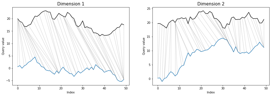
Differences between warping paths can be clearly seen at the twoway plots:

dtwPlot(shape_dtw_dependent_results, plot_type="twoway", xoffset=20)

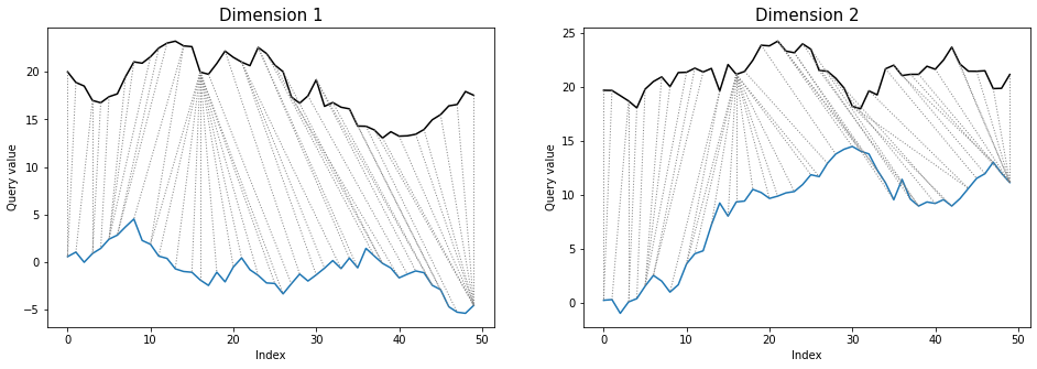
dtwPlot(shape_dtw_independent_results, plot_type="twoway", xoffset=20)

DTW parameters

For shape dtw we can use exactly the same additional parameters as for the dtw package. Below you can see see an example of specifying a sakoechiba window with a window size of 10:

import numpy as np
from numpy.random import randn
from shapedtw.shapedtw import shape_dtw
from shapedtw.dtwPlot import dtwPlot
from shapedtw.shapeDescriptors import SlopeDescriptor

np.random.seed(3)
ts_x = np.cumsum(randn(50))
ts_y = np.cumsum(randn(50))

slope_descriptor = SlopeDescriptor(slope_window=3)

shape_dtw_res = shape_dtw(
    x=ts_x,
    y=ts_y,
    subsequence_width=3,
    shape_descriptor=paa_descriptor,
    window_type="sakoechiba",
    window_args={"window_size": 10},
    keep_internals=True
)

dtwPlot(shape_dtw_res, plot_type="density")

Plots

We reused ploting mechanism from the dtw package in its core, however it was extended in order to allowing to plot multivariate shape dtw results as well.

In case of multivariate, dependent shape dtw the structure of both alignment and density plots look the same as in univariate version. The reason is that there is a single warping path, common for all dimensions. There are differences - comparing to univariate case - for twoway and threeway plots, as we want to show matching for all of time series dimensions. Therefore, instead of showing a single plot, we need to use a pyplot grid, containing as many plots as many dimensions time series has.

As for multivariate independent shape dtw, all types of plots require to use a pyplot grid. The reasin is that every single dimension has dedicated warping path, which we would like to show.

Plots - univariate case

As for univariate case, shape dtw plots are exactly the same as in case of dtw package. Let's calculate shape dtw for randomly generated time series:

import numpy as np
from numpy.random import randn
from shapedtw.shapedtw import shape_dtw
from shapedtw.dtwPlot import dtwPlot
from shapedtw.shapeDescriptors import SlopeDescriptor

np.random.seed(6)
ts_x = np.cumsum(randn(50))
ts_y = np.cumsum(randn(50))

slope_descriptor = SlopeDescriptor(slope_window=3)

shape_dtw_res = shape_dtw(
    x=ts_x,
    y=ts_y,
    subsequence_width=3,
    shape_descriptor=paa_descriptor,
    keep_internals=True
)

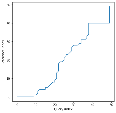
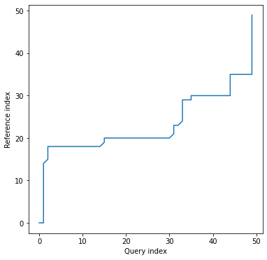
Alignment plot shows the alignment path between time series indices:

dtwPlot(shape_dtw_res, plot_type="alignment")

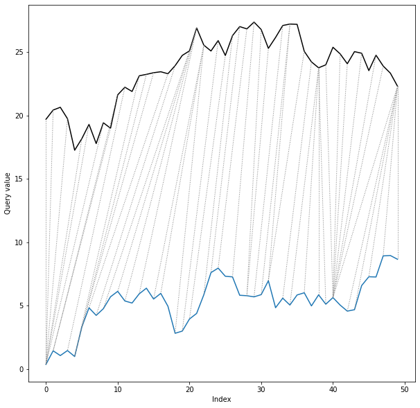
twoway plot displays time series values along with the alignment path:

dtwPlot(shape_dtw_res, plot_type="twoway", xoffset=20)

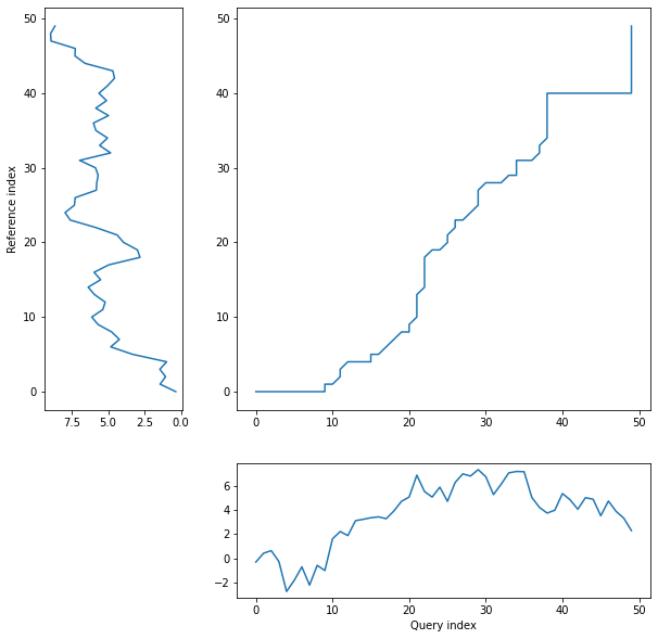
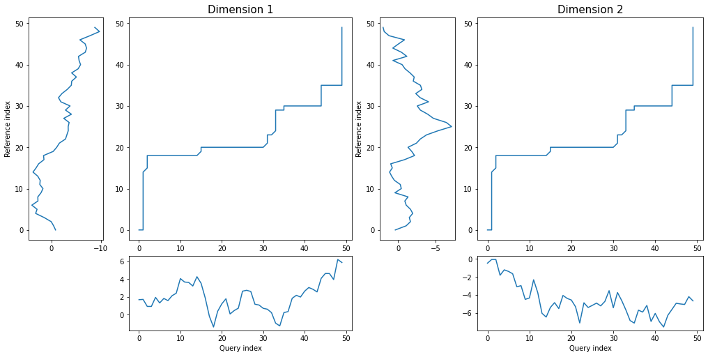
threeway plot displays query and reference time serience values against their warping curve:

dtwPlot(shape_dtw_res, plot_type="threeway")

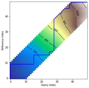
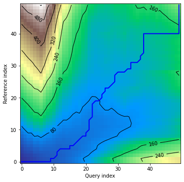
density plot displays distance matrix in visual form together with warping curve:

dtwPlot(shape_dtw_res, plot_type="density")

Plots - multivariate dependent variant

Let's define random, multidimensional time series:

import numpy as np
from numpy.random import randn
from shapedtw.shapedtw import shape_dtw
from shapedtw.dtwPlot import dtwPlot
from shapedtw.shapeDescriptors import SlopeDescriptor

np.random.seed(7)
ts_x = np.cumsum(randn(50, 2), axis=0)
ts_y = np.cumsum(randn(50, 2), axis=0)

slope_descriptor = SlopeDescriptor(slope_window=3)

shape_dtw_res = shape_dtw(
    x=ts_x,
    y=ts_y,
    subsequence_width=3,
    shape_descriptor=paa_descriptor,
    keep_internals=True,
    multivariate_version="dependent"
)

alignment plot looks exaclty the same as in case of univariate time series, since we've got one common warping path for all the dimensions:

dtwPlot(shape_dtw_res, plot_type="alignment")

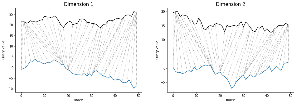
twoway plot shows all of time series dimensions and warping path:

dtwPlot(shape_dtw_res, plot_type="twoway", xoffset=20)

threeway plot displays both dimensions of query and reference series against warping curve:

dtwPlot(shape_dtw_res, plot_type="threeway")

density plot looks the same as in case of univariate time series, due to the fact that there is one common warping path:

dtwPlot(shape_dtw_res, plot_type="density")

Plots - multivariate independent variant

Let's define the same multidimensional time series as in previous example and calculate shape dtw results for them, but this time using independent multivariate version of the algorithm:

import numpy as np
from numpy.random import randn
from shapedtw.shapedtw import shape_dtw
from shapedtw.dtwPlot import dtwPlot
from shapedtw.shapeDescriptors import SlopeDescriptor

np.random.seed(7)
ts_x = np.cumsum(randn(50, 2), axis=0)
ts_y = np.cumsum(randn(50, 2), axis=0)

slope_descriptor = SlopeDescriptor(slope_window=3)

shape_dtw_res = shape_dtw(
    x=ts_x,
    y=ts_y,
    subsequence_width=3,
    shape_descriptor=paa_descriptor,
    keep_internals=True,
    multivariate_version="independent"
)

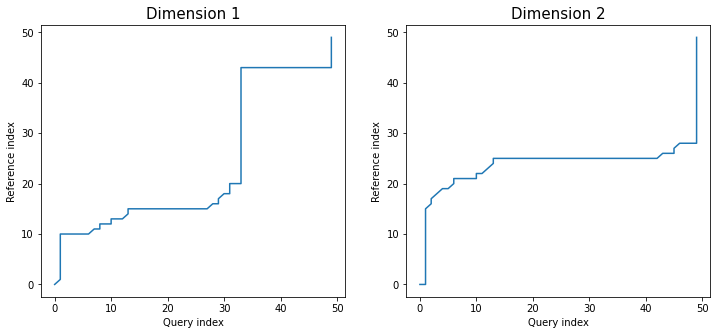
In this version alignment plot shows warping curves calculated for each dimension individually:

dtwPlot(shape_dtw_res, plot_type="alignment")

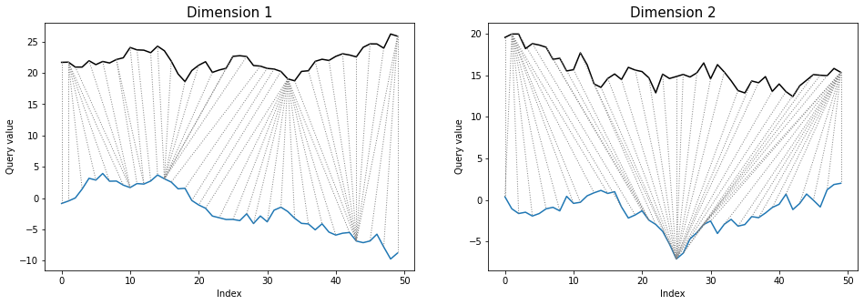
Similarly as in dependent version, twoway plot shows values of all dimensions with warping paths. This time each alignment path is different:

dtwPlot(shape_dtw_res, plot_type="twoway", xoffset=20)

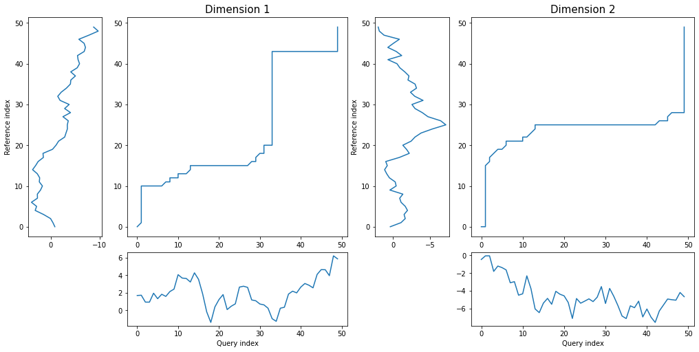
threeway plot also looks similarly as in multivariate dependent case:

dtwPlot(shape_dtw_res, plot_type="threeway")

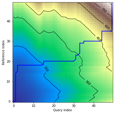
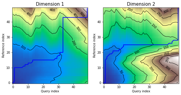
density plot displays as many distance matrices and warping curves as many dimensions time series has:

dtwPlot(shape_dtw_res, plot_type="density")

Applications

Shape dtw algorithm can be used wherever standard dtw is used; according to experiments conducted and described by Zhao and Itti shape dtw outperforms standard dtw variant in almost all cases.

As the author of this package, I think that the multidimensional version of shape dtw can be escpecially helpful for financiers and investors using technical analysis in their work. Since the algorithm takes into account the local shape of the time series, it can supports the process of finding similar formations from the past, also taking into account several securities or several technical analysis indicators simultaneously.

References

1. Giorgino, T., Computing and Visualizing Dynamic Time Warping Alignments in R: The dtw Package. J. Stat. Soft., doi:10.18637/jss.v031.i07.
2. Hu, B; Jin, H.; Keogh, E.; Shokoohi-Yekta, M., Generalizing DTW to the multi-dimensional case requires an adaptive approach, Data Mining and Knowledge Discovery, vol. 31, pp. 1–31, 2017. https://www.ncbi.nlm.nih.gov/pmc/articles/PMC5668684/
3. Itti, L.; Zhao, J., shapeDTW: shape Dynamic Time Warping, Pattern Recognition, Volume 74, pp. 171-184, Feb 2018. https://arxiv.org/pdf/1606.01601.pdf
4. Sakoe, H.; Chiba, S., Dynamic programming algorithm optimization for spoken word recognition, Acoustics, Speech, and Signal Processing, IEEE Transactions on , vol.26, no.1, pp. 43-49, Feb 1978. http://ieeexplore.ieee.org/xpls/abs_all.jsp?arnumber=1163055