thetafit

A simple python tool for Bayesian parameter estimation of nonlinear models, inspired by the mcmcstat MATLAB package.

Supports MAP estimation (optimization) and MCMC sampling via the Adaptive Metropolis (AM) algorithm.

The user supplies the function for calculating -2*log(likelihood), which, for Gaussian likelihood, amounts to calculating the sum of squares misfit between data and model.

A simple example is given below, for more examples see the demos folder.

Example: MONOD model

Let us fit the parameters theta = [a,b] of a simple model y = ax/(b+x) + N(0,sig2), describing bacterial growth.

1) Define model and data

First, we define the data and the sum of squares function. The function needs to be given in the form ssfun(theta,data), where theta is a dict of parameter name-value pairs, and data is an object of arbitrary form that contains typically the data and all other constants etc. that the function evaluation needs.

import numpy as np
import pandas as pd
from thetafit import Parameter, optimize, sample
from thetafit.utils import McmcOptions, jacob
import matplotlib.pyplot as plt

data = {
    'x': np.array([28., 55., 83., 110., 138., 225., 375.]),
    'y': np.array([0.053, 0.060, 0.112, 0.105, 0.099, 0.122, 0.125]),
    'sig2': 1.0,
}

modelfun = lambda theta, x: theta['a']*x/(theta['b']+x)
ssfun    = lambda theta, data: sum((data['y']-modelfun(theta, data['x']))**2/data['sig2'])

2) MAP estimation

Then, let us first minimize the sum of squares to get the MAP estimate. The initial values (with optional bounds) for the parameters are given as a list of Parameter objects. Here, we use a helper function for constructing such a list from the theta dict.

The optimization is called as optimize(ssfun, data, pars, **kwargs), where **kwargs are optional optimization configs fed to scipy.optimize, where one can choose the optimizer and its settings.

th0 = {'a': 0.15, 'b': 100}

params = lambda theta: [
    Parameter('a', init=theta['a'], target=True),
    Parameter('b', init=theta['b'], target=True)
]

thopt, res = optimize(ssfun, data, params(th0))
print(thopt)

which outputs the parameter values (and some information about the optimization process in res):

{'a': 0.14541945253897567, 'b': 49.05274598150096}

3) MCMC

Let us then do MCMC for the parameters, starting from the initial values obtained from the optimization. First, let us fix the error variance sig2 to the mean squared error (MSE) estimate:

mse = res.fun/(len(data['y'])-2)
data['sig2'] = mse

Then, we calculate the initial proposal covariance matrix via the Gauss-Newton Hessian approximation at the MAP estimate (note that a diagonal initial proposal covariance could be used as well, the adaptation will tune the proposal as the sampling proceeds).

J = jacob(modelfun, data['x'], params(thopt))
qcov = np.linalg.inv(J.T.dot(J))*mse

Then we define the options for the MCMC run via the McmcOptions object and perform the sampling:

options = McmcOptions(nsimu=4000, qcov=qcov, adaptint=100, printint=500)
res, chain, sschain = sample(ssfun, data, params(thopt), options)

which outputs the progress of the sampling:

Sampling these parameters:
name	start	[min,max]
a	0.14541945253897567	[-inf,inf]
b	49.05274598150096	[-inf,inf]
i: 500, rejected: 60.8%, out of bounds: 0.0%
i: 1000, rejected: 62.6%, out of bounds: 0.0%
i: 1500, rejected: 63.8%, out of bounds: 0.0%
i: 2000, rejected: 64.3%, out of bounds: 0.0%
i: 2500, rejected: 64.9%, out of bounds: 0.0%
i: 3000, rejected: 65.5%, out of bounds: 0.0%
i: 3500, rejected: 65.8%, out of bounds: 0.0%

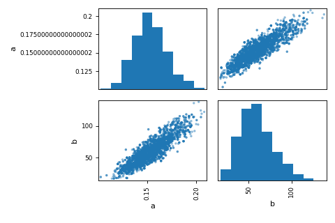
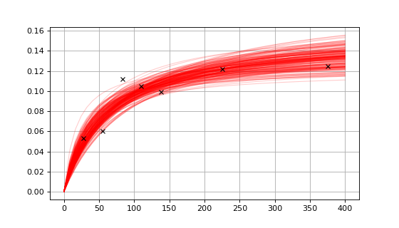
Then, let us visualize the results:

pd.plotting.scatter_matrix(chain)

xplot = np.linspace(0,400)
preds = np.stack([modelfun(chain.loc[i], xplot) for i in range(2000,4000,10)])

plt.figure(figsize=(7,4))
plt.plot(xplot, preds.T, 'r-', lw=1, alpha=0.2)
plt.plot(data['x'], data['y'], 'kx')
plt.grid(True)
plt.show()