A python package for causal inference

Project description

YLearn, a pun of "learn why", is a python package for causal inference which supports various aspects of causal inference ranging from causal effect identification, estimation, and causal graph discovery, etc.
Documentation website: https://ylearn.readthedocs.io
中文文档地址:https://ylearn.readthedocs.io/zh_CN/latest/
Installation
Pip
The simplest way of installing YLearn is using pip:
pip install ylearn
Note that Graphviz is required to plot causal graph in notebook, so install it before running YLearn. See https://graphviz.org/download/ for more details about Graphviz installation.
Conda
YLearn can also be installed with conda. Install it from the channel conda-forge:
conda install -c conda-forge ylearn
This will install YLearn and all requirements including Graphviz.
Docker
We also publish an image in Docker Hub which can be downloaded directly and includes the components:
- Python 3.8
- YLearn and its dependent packages
- JupyterLab
Download the docker image:
docker pull datacanvas/ylearn
Run a docker container:
docker run -ti -e NotebookToken="your-token" -p 8888:8888 datacanvas/ylearn
Then one can visit http://<ip-addr>:8888 in the browser and type in the token to start.
Overview of YLearn
Machine learning has made great achievements in recent years. The areas in which machine learning succeeds are mainly for prediction, e.g., the classification of pictures of cats and dogs. However, machine learning is incapable of answering some questions that naturally arise in many scenarios. One example is for the counterfactual questions in policy evaluations: what would have happened if the policy had changed? Due to the fact that these counterfactuals can not be observed, machine learning models, the prediction tools, can not be used. These incapabilities of machine learning partly give rise to applications of causal inference in these days.
Causal inference directly models the outcome of interventions and formalizes the counterfactual reasoning. With the aid of machine learning, causal inference can draw causal conclusions from observational data in various manners nowadays, rather than relying on conducting craftly designed experiments.
A typical complete causal inference procedure is composed of three parts. First, it learns causal relationships using the technique called causal discovery. These relationships are then expressed either in the form of Structural Causal Models or Directed Acyclic Graphs (DAG). Second, it expresses the causal estimands, which are clarified by the interested causal questions such as the average treatment effects, in terms of the observed data. This process is known as identification. Finally, once the causal estimand is identified, causal inference proceeds to focus on estimating the causal estimand from observational data. Then policy evaluation problems and counterfactual questions can also be answered.
YLearn, equipped with many techniques developed in recent literatures, is implemented to support the whole causal inference pipeline from causal discovery to causal estimand estimation with the help of machine learning. This is more promising especially when there are abundant observational data.
Concepts in YLearn

There are 5 main concepts in YLearn corresponding to the causal inference pipeline.
-
CausalDiscovery. Discovering the causal relationships in the observational data.
-
CausalModel. Representing the causal relationships in the form of
CausalGraphand doing other related operations such as identification withCausalModel. -
EstimatorModel. Estimating the causal estimand with various techniques.
-
Policy. Selecting the best policy for each individual.
-
Interpreter. Explaining the causal effects and polices.
These components are connected to give a full pipeline of causal inference, which are also encapsulated into a single API Why.
Pipeline in YLearn
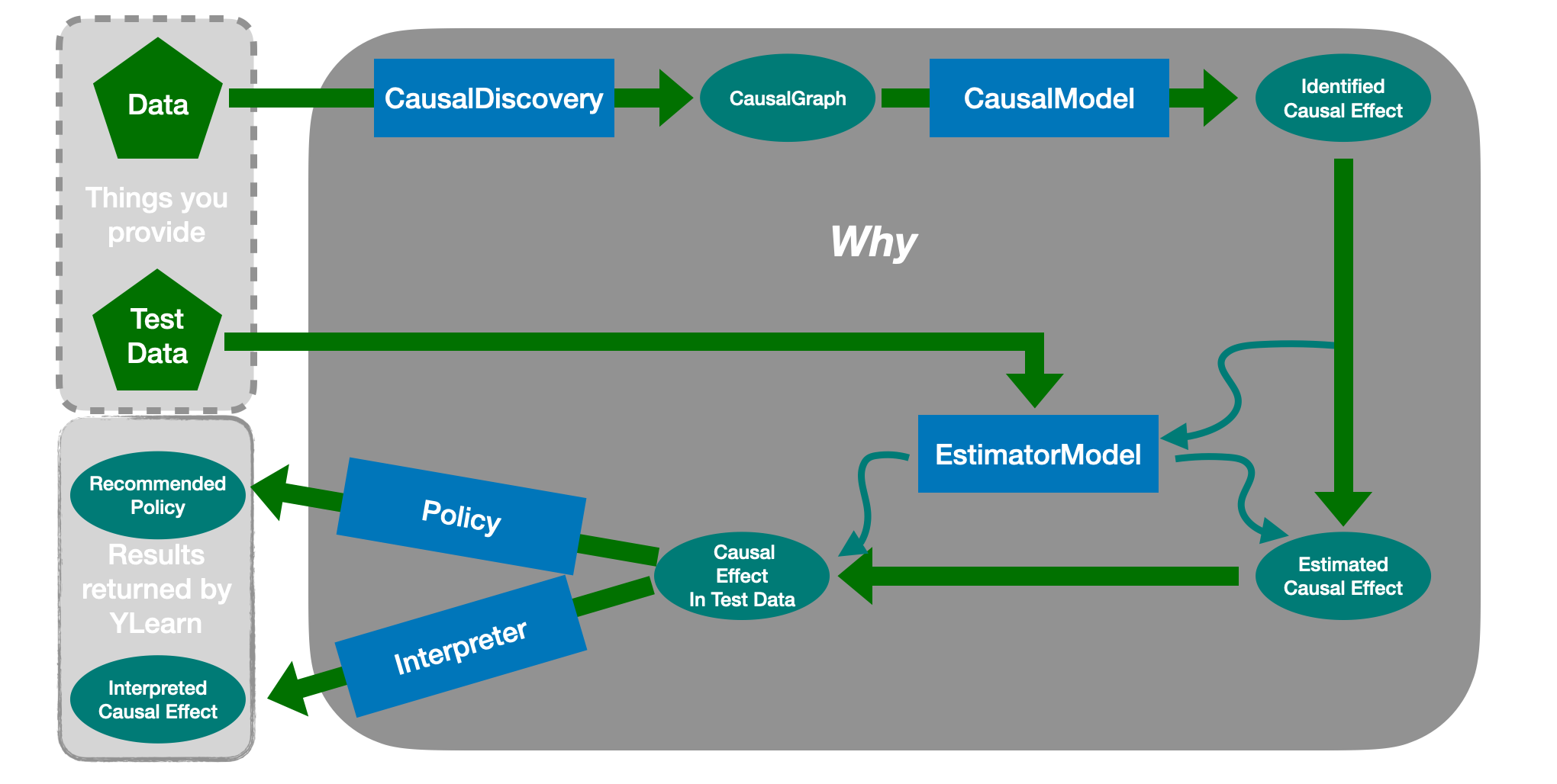
Starting from the training data:
- One first uses the
CausalDiscoveryto reveal the causal structures in data, which will usually output aCausalGraph. - The causal graph is then passed into the
CausalModel, where the interested causal effects are identified and converted into statistical estimands. - An
EstimatorModelis then trained with the training data to model relationships between causal effects and other variables, i.e., estimating causal effects in training data. - One can then use the trained
EstimatorModelto predict causal effects in some new test dataset and evaluate the policy assigned to each individual or interpret the estimated causal effects.
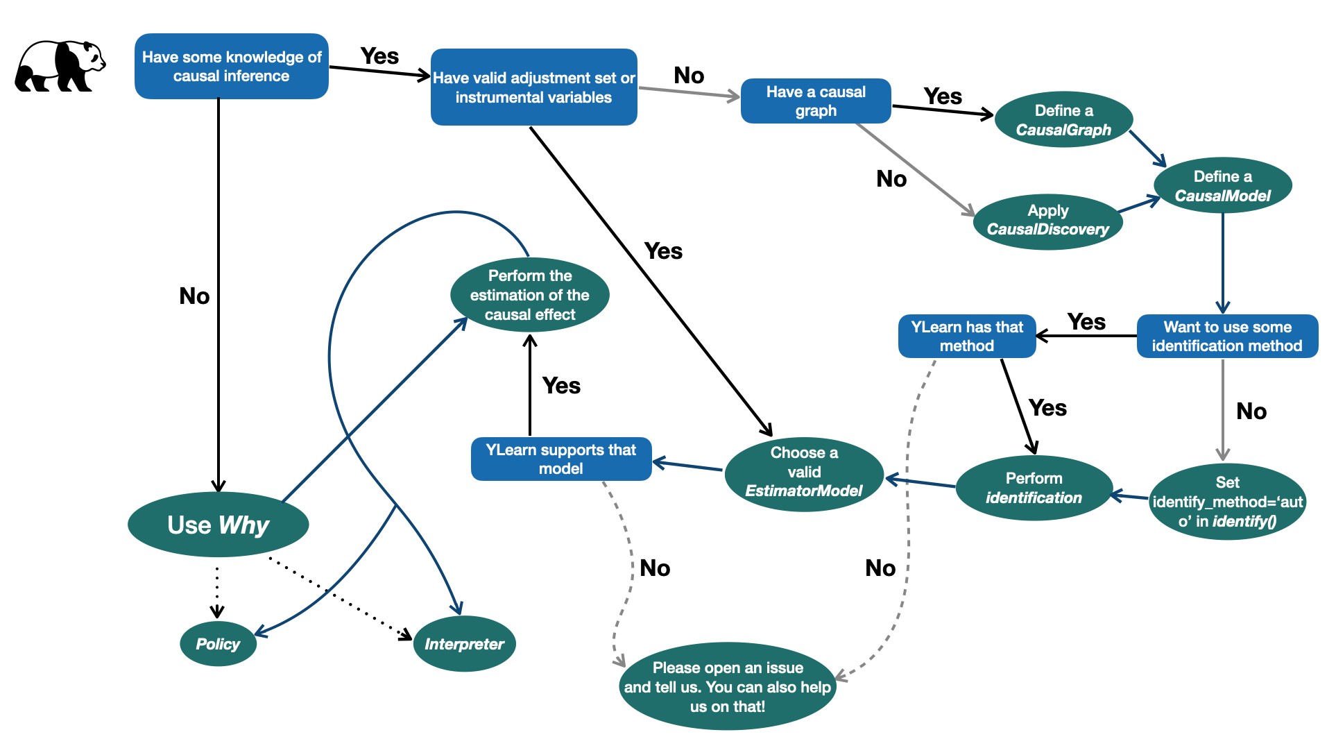
It is also helpful to use the following flow chart in many causal inference tasks
Quick Start
In this part, we first show several simple example usages of YLearn. These examples cover the most common functionalities. Then we present a case stuy with Why to unveil the hidden
causal relations in data.
Example usages
We present several necessary example usages of YLearn in this section, which covers defining a causal graph, identifying the causal effect, and training an estimator model, etc. Please see their specific documentations for more details.
-
Representation of the causal graph
Given a set of variables, the representation of its causal graph in YLearn requires a python
dictto denote the causal relations of variables, in which the keys of thedictare children of all elements in the corresponding values where each value usually should be a list of names of variables. For an instance, in the simplest case, for a given causal graphX <- W -> Y, we first define a pythondictfor the causal relations, which will then be passed toCausalGraphas a parameter:causation = {'X': ['W'], 'W':[], 'Y':['W']} cg = CausalGraph(causation=causation)
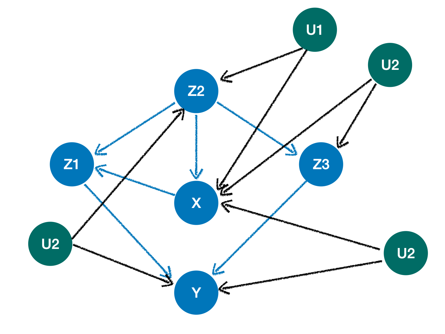
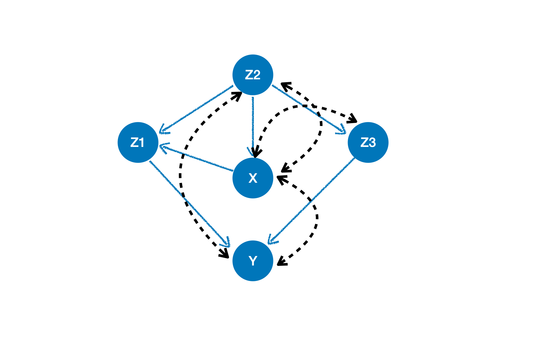
cgwill be the causal graph encoding the causal relationX <- W -> Yin YLearn. If there exist unobserved confounders in the causal graph, then, aside from the observed variables, we should also define a pythonlistcontaining these causal relations. For example, a causal graph with unobserved confounders (green nodes)is first converted into a graph with latent confounding arcs (black dotted llines with two directions)
To represent such causal graph, we should
(1) define a python
dictto represent the observed parts, and(2) define a
listto encode the latent confounding arcs where each element in thelistincludes the names of the start node and the end node of a latent confounding arc:from ylearn.causal_model.graph import CausalGraph # define the dict to represent the observed parts causation_unob = { 'X': ['Z2'], 'Z1': ['X', 'Z2'], 'Y': ['Z1', 'Z3'], 'Z3': ['Z2'], 'Z2': [], } # define the list to encode the latent confounding arcs for unobserved confounders arcs = [('X', 'Z2'), ('X', 'Z3'), ('X', 'Y'), ('Z2', 'Y')] cg_unob = CausalGraph(causation=causation_unob, latent_confounding_arcs=arcs)
-
Identification of causal effect
It is crucial to identify the causal effect when we want to estimate it from data. The first step for identifying the causal effect is identifying the causal estimand. This can be easily done in YLearn. For an instance, suppose that we are interested in identifying the causal estimand
P(Y|do(X=x))in the causal graphcgdefined above, then we can simply define an instance ofCausalModeland call theidentify()method:cm = CausalModel(causal_graph=cg) cm.identify(treatment={'X'}, outcome={'Y'}, identify_method=('backdoor', 'simple'))
where we use the backdoor-adjustment method here by specifying
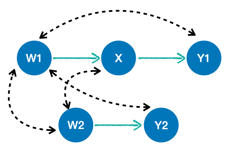
identify_method=('backdoor', 'simple'). YLearn also supports front-door adjustment, finding instrumental variables, and, most importantly, the general identification method developed in [1] which is able to identify any causal effect if it is identifiable. For an example, given the following causal graph,if we want to identify
P(Y1, Y2|do(X)), racalling that black dotted lines with two directions are latent confounding arcs (i.e., there is an unobserved confounder pointing to the two end nodes of each black dotted line), we can apply YLearn as followscausation = { 'W1': [], 'W2': [], 'X': ['W1'], 'Y1': ['X'], 'Y2': ['W2'] } arcs = [('W1', 'Y1'), ('W1', 'W2'), ('W1', 'Y2'), ('W1', 'Y1')] cg = graph.CausalGraph(causation, latent_confounding_arcs=arcs) cm = model.CausalModel(cg) p = cm.id({'Y1', 'Y2'}, {'X'}) p.show_latex_expression()
which will give us the identified causal effect
P(Y1, Y2|X)as followsand calling the method
p.parse()will give us the latex expression\sum_{W2}\left[\left[P(Y2|W2)\right]\right]\left[\sum_{W1}\left[P(W1)\right]\left[P(Y1|X, W1)\right]\right]\left[P(W2)\right] -
Instrumental variables
Instrumental variable is an important technique in causal inference. The approach of using YLearn to find valid instrumental variables is very straightforward. For example, suppose that we have a causal graph
,
we can follow the common procedure of utilizing identify methods of
CausalModelto find the instrumental variables: (1) define thedictandlistof the causal relations; (2) define an instance ofCausalGraphto build the related causal graph in YLearn; (3) define an instance ofCausalModelwith the instance ofCausalGraphin last step being the input; (4) call theget_iv()method ofCausalModelto find the instrumental variablescausation = { 'p': [], 't': ['p', 'l'], 'l': [], 'g': ['t', 'l'] } arc = [('t', 'g')] cg = CausalGraph(causation=causation, latent_confounding_arcs=arc) cm = CausalModel(causal_graph=cg) cm.get_iv('t', 'g')
-
Estimation of causal effect
The estimation of causal effects in YLearn is also fairly easy. It follows the common approach of deploying a machine learning model since YLearn focuses on the intersection of machine learning and causal inference in this part. Given a dataset, one can apply any
EstimatorModelin YLearn with a procedure composed of 3 distinct steps:- Given data in the form of
pandas.DataFrame, find the names oftreatment, outcome, adjustment, covariate. - Call
fit()method ofEstimatorModelto train the model with the names of treatment, outcome, and adjustment specified in the first step. - Call
estimate()method ofEstimatorModelto estimate causal effects in test data.
One can refer to the documentation website for methodologies of many estimator models implemented by YLearn.
- Given data in the form of
-
Using the all-in-one API: Why
For the purpose of applying YLearn in a unified and easier manner, YLearn provides the API
Why.Whyis an API which encapsulates almost everything in YLearn, such as identifying causal effects and scoring a trained estimator model. To useWhy, one should first create an instance ofWhywhich needs to be trained by calling its methodfit(), after which other utilities, such ascausal_effect(),score(), andwhatif(), can be used. This procedure is illustrated in the following code example:from sklearn.datasets import fetch_california_housing from ylearn import Why housing = fetch_california_housing(as_frame=True) data = housing.frame outcome = housing.target_names[0] data[outcome] = housing.target why = Why() why.fit(data, outcome, treatment=['AveBedrms', 'AveRooms']) print(why.causal_effect())

Case Study
In the notebook CaseStudy, we utilize a typical bank customer dataset to further demonstrate the usage of the all-in-one API Why of YLearn. Why covers the full processing pipeline of causal learning, including causal discovery, causal effect identification, causal effect estimation, counterfactual inference, and policy learning. Please refer to CaseStudy for more details.
Contributing
We welcome community contributors to the project. Before you start, please firstly read our code of conduct and contributing guidelines.
Communication
We provide several communcication channels for developers.
- GitHub Issues and Discussions
- Email: ylearn@zetyun.com
- Slack Workspace
License
See the LICENSE file for license rights and limitations (Apache-2.0).
References
[1] J. Pearl. Causality: models, reasoing, and inference.
[2] S. Shpister and J. Identification of Joint Interventional Distributions in Recursive Semi-Markovian Causal Models. AAAI 2006.
[3] B. Neal. Introduction to Causal Inference.
[4] M. Funk, et al. Doubly Robust Estimation of Causal Effects. Am J Epidemiol. 2011 Apr 1;173(7):761-7.
[5] V. Chernozhukov, et al. Double Machine Learning for Treatment and Causal Parameters. arXiv:1608.00060.
[6] S. Athey and G. Imbens. Recursive Partitioning for Heterogeneous Causal Effects. arXiv: 1504.01132.
[7] A. Schuler, et al. A comparison of methods for model selection when estimating individual treatment effects. arXiv:1804.05146.
[8] X. Nie, et al. Quasi-Oracle estimation of heterogeneous treatment effects. arXiv: 1712.04912.
[9] J. Hartford, et al. Deep IV: A Flexible Approach for Counterfactual Prediction. ICML 2017.
[10] W. Newey and J. Powell. Instrumental Variable Estimation of Nonparametric Models. Econometrica 71, no. 5 (2003): 1565–78.
[11] S. Kunzel2019, et al. Meta-Learners for Estimating Heterogeneous Treatment Effects using Machine Learning. arXiv: 1706.03461.
[12] J. Angrist, et al. Identification of causal effects using instrumental variables. Journal of the American Statistical Association.
[13] S. Athey and S. Wager. Policy Learning with Observational Data. arXiv: 1702.02896.
[14] P. Spirtes, et al. Causation, Prediction, and Search.
[15] X. Zheng, et al. DAGs with NO TEARS: Continuous Optimization for Structure Learning. arXiv: 1803.01422.
Release history Release notifications | RSS feed


Download files
Download the file for your platform. If you're not sure which to choose, learn more about installing packages.
Source Distribution
Built Distributions
Hashes for ylearn-0.2.0-cp311-cp311-win_amd64.whl
| Algorithm | Hash digest | |
|---|---|---|
| SHA256 | b6a3237f3dfeb49e7fd3f382b06fbece121e05bc308500e37d28dab9b3d70a0f |
|
| MD5 | 11b10d18ea9872174c260c9874be9a98 |
|
| BLAKE2b-256 | 0bff4f5c256565411a522b1cbfd58eb116126994363ecfa8c1085a8a9e226d2c |
Hashes for ylearn-0.2.0-cp311-cp311-manylinux_2_17_x86_64.manylinux2014_x86_64.whl
| Algorithm | Hash digest | |
|---|---|---|
| SHA256 | 491cf056e99d8ae4e76650039e803398b1e379cfbc2ca8b8f6da0cf8d1fc24b0 |
|
| MD5 | 22921900b5f2384b708bbec7c09295f7 |
|
| BLAKE2b-256 | dec489e01338f46722273dbd3d8c09ffb241c9dc724a5773ee6374a5f468a7cd |
Hashes for ylearn-0.2.0-cp311-cp311-macosx_10_9_universal2.whl
| Algorithm | Hash digest | |
|---|---|---|
| SHA256 | 8ad79be7dffce71e365d7e5c73ecac385a7f8854619ca80e64d1f64b427dcd62 |
|
| MD5 | cc314e4cb7878c27a9e39de5899f6893 |
|
| BLAKE2b-256 | f432d651a4bea9e8d0abeed854b01cbf6110710d035b8f17d845856949e5e567 |
Hashes for ylearn-0.2.0-cp310-cp310-win_amd64.whl
| Algorithm | Hash digest | |
|---|---|---|
| SHA256 | 145d51a32647defbce655e88b3c4ade55868359e8bf7c202649b86aef196937a |
|
| MD5 | 2d92b75b5746f54573f3d9af8a9b0331 |
|
| BLAKE2b-256 | db41efc9acf66a43a62e83e488d9463d78236388103cfbb056b58e9f75256d79 |
Hashes for ylearn-0.2.0-cp310-cp310-manylinux_2_17_x86_64.manylinux2014_x86_64.whl
| Algorithm | Hash digest | |
|---|---|---|
| SHA256 | ca91f120b419543c92bcb966daa0b1d85b923378148953c9cd45627a3a539d33 |
|
| MD5 | b7abfb42a9dd9b4f0dd737a2defe5a2c |
|
| BLAKE2b-256 | f4f3c0e9b82fd4ecde367e4b74f1d263be530c1ff2f490d37f99ac1ecc6d446f |
Hashes for ylearn-0.2.0-cp310-cp310-macosx_11_0_x86_64.whl
| Algorithm | Hash digest | |
|---|---|---|
| SHA256 | 1079749d2b2bea654bd5dc222c38f058127037eb333e1e188dcc2f82881b98ca |
|
| MD5 | e1f1892615dea19032ae0ee36bdd65bb |
|
| BLAKE2b-256 | 866a0adfed3cff2a923202a92b619d0169a9def582f0160dab6eeac140671888 |
Hashes for ylearn-0.2.0-cp39-cp39-win_amd64.whl
| Algorithm | Hash digest | |
|---|---|---|
| SHA256 | 61d9d9aca1a40e29334f967c064d036dbbb9f1e744dde1fa85594f0f4e888c37 |
|
| MD5 | ad81e5b228deac238634f648df00cd15 |
|
| BLAKE2b-256 | 500ea9c18c19c109f43eae282dd73e4094f8060dab72515a48098446594e87be |
Hashes for ylearn-0.2.0-cp39-cp39-manylinux_2_17_x86_64.manylinux2014_x86_64.whl
| Algorithm | Hash digest | |
|---|---|---|
| SHA256 | 4a7234f29b06ed6f8a0985c3300b86884cbc213144fc8718002a29b802faf475 |
|
| MD5 | 898e3db1a9401b8f9b5719418c93ec17 |
|
| BLAKE2b-256 | 27c48dd7852d9937bf67c9b38928f8cca92fb07e4f805267fd798b7e01d9b9db |
Hashes for ylearn-0.2.0-cp39-cp39-macosx_11_0_x86_64.whl
| Algorithm | Hash digest | |
|---|---|---|
| SHA256 | e900d9005bc597175bb78d58869130f6e411ed5edcb504311c8adb9acd9ef834 |
|
| MD5 | 7c58e7238b8afe28e7fd5ecdc79a0a42 |
|
| BLAKE2b-256 | 4f360e244a4c9bba63e64c2c0c1d86cc563a69c1f7b2bcbaa0cf0ec9affb26bb |
Hashes for ylearn-0.2.0-cp38-cp38-win_amd64.whl
| Algorithm | Hash digest | |
|---|---|---|
| SHA256 | 0ef4142ad76dd869c7ee467a997c1ce079b54278016b7ca56e68c37fab91d3fe |
|
| MD5 | 0a6bb4d18690eac0fdd5ae48a3b6a993 |
|
| BLAKE2b-256 | d4d82f2881bd0b138a05ce38affc82980fb993b9296d22575b5a0afa4adfca29 |
Hashes for ylearn-0.2.0-cp38-cp38-manylinux_2_17_x86_64.manylinux2014_x86_64.whl
| Algorithm | Hash digest | |
|---|---|---|
| SHA256 | 88b1dfb1f2275e8283a79b51442f11b8c2dd99dd6e32de67cf17718ffab30f0a |
|
| MD5 | 2a79557ec3b4f0264b214a313df9ba76 |
|
| BLAKE2b-256 | 980d5720cfaa51f6c8a3f69342f17b9388258dba8e0f37d9d71abf23650b1eb2 |
Hashes for ylearn-0.2.0-cp38-cp38-macosx_10_15_x86_64.whl
| Algorithm | Hash digest | |
|---|---|---|
| SHA256 | d5c9d13110319879abecf7559a4675128bd502b2d3bf9c3fedb988cdb73d20ad |
|
| MD5 | 33e1e35b18ca92f9b4b4b962c11c4970 |
|
| BLAKE2b-256 | fdc563d108d11c54499281e5bb0b1d7811a4f5b82837a973c24cfac7609c542c |
Hashes for ylearn-0.2.0-cp37-cp37m-win_amd64.whl
| Algorithm | Hash digest | |
|---|---|---|
| SHA256 | 22335cbf6c77b60f03a051606c0fc766c83c7670c674c1a8b477f6532a03640b |
|
| MD5 | 13ed6d6ac914e1c44cfae96084e4af23 |
|
| BLAKE2b-256 | 54c6ba62ec9a94a7f02f57d90ece891e3c1a5d502418e9f65b34ffb542990939 |
Hashes for ylearn-0.2.0-cp37-cp37m-manylinux_2_17_x86_64.manylinux2014_x86_64.whl
| Algorithm | Hash digest | |
|---|---|---|
| SHA256 | 5d387796ce101921a40884193d27267f3792fee24bf7909703d4a85ebc7aafe9 |
|
| MD5 | 5a35b1d07a05eeb224a25859c3e35309 |
|
| BLAKE2b-256 | 3eb7a222c8252b7f94a94fa09c5f64c5830a56f9dde11a3941789a334d121558 |
Hashes for ylearn-0.2.0-cp37-cp37m-macosx_10_15_x86_64.whl
| Algorithm | Hash digest | |
|---|---|---|
| SHA256 | 46cf2b0a7f47f16cff5281ee2b0bda6f0c8544dd85aceb10782fc63439b5310c |
|
| MD5 | c0d020379c875e13bdcfd903eb518f33 |
|
| BLAKE2b-256 | dbcfb97d576db9d7e453a0af064c3c624587439d6971c2280919e3f6e27a3878 |
Hashes for ylearn-0.2.0-cp36-cp36m-manylinux_2_17_x86_64.manylinux2014_x86_64.whl
| Algorithm | Hash digest | |
|---|---|---|
| SHA256 | 78c10b8f0c923b05a4003ab51a130f67c0de024668f96e5e86cc21bf4882d93f |
|
| MD5 | d29da6efcbb43ef03ac51b4a63c4ed0e |
|
| BLAKE2b-256 | f839c2d46f90e866d580cbab386f103dcc50adb8130770d8826eb30f1ae6bc8b |
Hashes for ylearn-0.2.0-cp36-cp36m-macosx_10_14_x86_64.whl
| Algorithm | Hash digest | |
|---|---|---|
| SHA256 | 4942731194741a0928379ccc085bc62e93bf788d822f32bc13f2cf1638042dc4 |
|
| MD5 | 6f07cf73b9932d78f69ff8b380b3c91f |
|
| BLAKE2b-256 | a293a297d0490e836f1c4feb347aa849dd75ff0ac42329e53144c509cac511cc |


