Python binding for odeiv2 in GNU Scientific Library (GSL).

Project description


pygslodeiv2 provides a Python binding to the Ordinary Differential Equation integration routines exposed by the odeiv2 interface of GSL - GNU Scientific Library. The odeiv2 interface allows a user to numerically integrate (systems of) differential equations.
The following stepping functions are available:
rk2
rk4
rkf45
rkck
rk8pd
rk1imp
rk2imp
rk4imp
bsimp
msadams
msbdf
Note that all implicit steppers (those ending with “imp”) and msbdf require a user supplied callback for calculating the jacobian.
You may also want to know that you can use pygslodeiv2 from pyodesys which can e.g. derive the Jacobian analytically (using SymPy). pyodesys also provides plotting functions, C++ code-generation and more.
Documentation
Autogenerated API documentation for latest stable release is found here: https://bjodah.github.io/pygslodeiv2/latest (and the development version for the current master branch are found here: http://hera.physchem.kth.se/~pygslodeiv2/branches/master/html).
Installation
Simplest way to install is to use the conda package manager:
$ conda install -c conda-forge pygslodeiv2 pytest
$ python -m pytest --pyargs pygslodeiv2
tests should pass.
Binary distribution is available here: https://anaconda.org/bjodah/pygslodeiv2, conda recipes for stable releases are available here: http://hera.physchem.kth.se/~pygslodeiv2/conda-recipes.
Source distribution is available here (requires GSL v1.16 or v2.1 shared lib with headers): https://pypi.python.org/pypi/pygslodeiv2 (with mirrored files kept here: http://hera.physchem.kth.se/~pygslodeiv2/releases)
Examples
The classic van der Pol oscillator (see examples/van_der_pol.py)
>>> import numpy as np
>>> from pygslodeiv2 import integrate_predefined  # also: integrate_adaptive
>>> mu = 1.0
>>> def f(t, y, dydt):
...     dydt[0] = y[1]
...     dydt[1] = -y[0] + mu*y[1]*(1 - y[0]**2)
...
>>> def j(t, y, Jmat, dfdt):
...     Jmat[0, 0] = 0
...     Jmat[0, 1] = 1
...     Jmat[1, 0] = -1 -mu*2*y[1]*y[0]
...     Jmat[1, 1] = mu*(1 - y[0]**2)
...     dfdt[0] = 0
...     dfdt[1] = 0
...
>>> y0 = [1, 0]; dt0=1e-8; t0=0.0; atol=1e-8; rtol=1e-8
>>> tout = np.linspace(0, 10.0, 200)
>>> yout, info = integrate_predefined(f, j, y0, tout, dt0, atol, rtol,
...                                   method='bsimp')  # Implicit Bulirsch-Stoer
>>> import matplotlib.pyplot as plt
>>> series = plt.plot(tout, yout)
>>> plt.show()  # doctest: +SKIP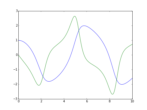
For more examples see examples/, and rendered jupyter notebooks here: http://hera.physchem.kth.se/~pygslodeiv2/branches/master/examples
License
The source code is Open Source and is released under GNU GPL v3. See LICENSE for further details. Contributors are welcome to suggest improvements at https://github.com/bjodah/pygslodeiv2


