Quantum Signal Processing

Introduction

Quantum signal processing is a framework for quantum algorithms including Hamiltonian simulation, quantum linear system solving, amplitude amplification, etc.

Quantum signal processing performs spectral transformation of any unitary U, given access to an ancilla qubit, a controlled version of U and single-qubit rotations on the ancilla qubit. It first truncates an arbitrary spectral transformation function into a Laurent polynomial, then finds a way to decompose the Laurent polynomial into a sequence of products of controlled-U and single qubit rotations (by certain "QSP phase angles") on the ancilla. Such routines achieve optimal gate complexity for many of the quantum algorithmic tasks mentioned above. The task achieved is essentially entirely defined by the QSP phase angles employed in the QSP operation sequence, and as such a central part is finding these QSP phase angles, given the desired Laurent polynomial.

This python package generates QSP phase angles using the code based on two different methods. The "laurent" method employs Finding Angles for Quantum Signal Processing with Machine Precision, and extends the original code for QSP phase angle calculation, at https://github.com/alibaba-edu/angle-sequence. The "tf" method employs tensorflow + keras, and finds the QSP angles using optimization.

QSP conventions

As described in A Grand Unification of Quantum Algorithms, two important QSP model conventions used in the literature are known as Wx, where the signal W(a) is an X-rotation and QSP signal processing phase shifts are Z-rotations, and Wz, where the signal W(a) is a Z-rotation and QSP signal processing phase shifts are X-rotations.

Specifically, in the Wx convention, the QSP operation sequence is:

And in the Wz convention, the QSP operation sequence is:

They are related by a Hadamard transform:

The Wz convention is convenient for and employed in Laurent polynomial formulations of QSP, whereas the Wx convention is more traditional, e.g. as employed in quantum singular value transform applications of QSP.

This package can generate QSP phase angles for both conventions (whereas earlier code only handled the Wz convention). The challenge is that if one wants a certain polynomial in the Wx convention, one cannot just use the phases generated for this polynomial in the Wz convention. Instead, first the Q_x(a) corresponding to P_x(a) is needed to complete the full U_x. This then gives . Computing the QSP phases for P_z(a) in the Wz convention then gives the desired QSP phases for P_x(a) in the Wx convention, if suitable care is taken with respect to the Q(a) polynomial.

In addition to specifying the signal rotation operator W and the signal processing operator phase shifts, the QSP signal basis must also be specified. In this code, the default basis is |+>, but the code also allows the |0> basis to be used (when using tensorflow optimization to generate the phase angles). See the "--measurement" option.

Examples

This package also plots the QSP response function, and can be run from the command line. In the example below, the blue line shows the target ideal polynomial QSP response function P_x(a); the red line shows the real part of the response achieved by the QSP phases, and the green line shows the imaginary part of the QSP response, with L=20.

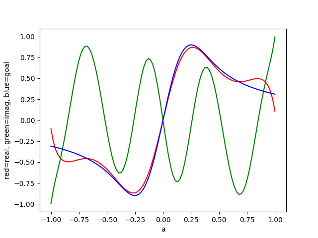
This was generated by running pyqsp --plot invert, which generated the following text output:

b=20, j0=10
[PolyOneOverX] minimum [-2.90002589] is at [-0.25174082]: normalizing
Laurent P poly 0.0002108924030879319 * w ^ (-21) + -0.0006894043260278334 * w ^ (-19) + 0.001994436843136674 * w ^ (-17) + -0.005148265426149545 * w ^ (-15) + 0.011941126989562179 * w ^ (-13) + -0.02504164571900347 * w ^ (-11) + 0.04774921151669176 * w ^ (-9) + -0.08322978307559126 * w ^ (-7) + 0.1333200017468883 * w ^ (-5) + -0.1973241700493915 * w ^ (-3) + 0.2714342596621151 * w ^ (-1) + 0.2714342596621151 * w ^ (1) + -0.1973241700493915 * w ^ (3) + 0.1333200017468883 * w ^ (5) + -0.08322978307559126 * w ^ (7) + 0.04774921151669176 * w ^ (9) + -0.02504164571900347 * w ^ (11) + 0.011941126989562179 * w ^ (13) + -0.005148265426149545 * w ^ (15) + 0.001994436843136674 * w ^ (17) + -0.0006894043260278334 * w ^ (19) + 0.0002108924030879319 * w ^ (21)
Laurent Q poly -2.784691352688532e-05 * w ^ (-21) + -3.467046922689296e-06 * w ^ (-19) + -0.00023447352272530086 * w ^ (-17) + 0.00018731079814912242 * w ^ (-15) + -0.0007159634932856078 * w ^ (-13) + 0.0032821300323626736 * w ^ (-11) + -0.001907488898700853 * w ^ (-9) + 0.012591630667616198 * w ^ (-7) + -0.02371053103573988 * w ^ (-5) + -0.016629567619072996 * w ^ (-3) + -0.18519029619384528 * w ^ (-1) + -0.20476480667058175 * w ^ (1) + -0.5374170003848409 * w ^ (3) + -0.2638332742746844 * w ^ (5) + 0.21212227077358078 * w ^ (7) + 0.27748656462486654 * w ^ (9) + -0.34978762979573563 * w ^ (11) + 0.17888109364117422 * w ^ (13) + -0.07649917245226195 * w ^ (15) + 0.03551004671728361 * w ^ (17) + -0.011926352140796492 * w ^ (19) + 0.001997855069006951 * w ^ (21)
Laurent Pprime poly 0.00018304548956104657 * w ^ (-21) + -0.0006928713729505227 * w ^ (-19) + 0.001759963320411373 * w ^ (-17) + -0.0049609546280004226 * w ^ (-15) + 0.01122516349627657 * w ^ (-13) + -0.021759515686640796 * w ^ (-11) + 0.0458417226179909 * w ^ (-9) + -0.07063815240797505 * w ^ (-7) + 0.10960947071114842 * w ^ (-5) + -0.2139537376684645 * w ^ (-3) + 0.08624396346826982 * w ^ (-1) + 0.06666945299153335 * w ^ (1) + -0.7347411704342324 * w ^ (3) + -0.1305132725277961 * w ^ (5) + 0.12889248769798953 * w ^ (7) + 0.3252357761415583 * w ^ (9) + -0.3748292755147391 * w ^ (11) + 0.1908222206307364 * w ^ (13) + -0.0816474378784115 * w ^ (15) + 0.037504483560420285 * w ^ (17) + -0.012615756466824325 * w ^ (19) + 0.0022087474720948828 * w ^ (21)
[QuantumSignalProcessingWxPhases] Error in reconstruction from QSP angles = 0.4862234440482484
QSP angles = [0.11177647198529908, 0.321286291382733, -2.449109005349844, 0.5475854935639934, -0.23068701778999645, 1.852723853663707, -0.1638598380129409, -0.031620025684050396, -0.3018780297835489, -1.8740083256355018, 0.6314873861312269, -0.036881744534211114, 1.300525766122238, 0.3073180685644643, -0.23974313142278042, 0.09536754986888613, -1.188342341212731, -0.6092537117168764, 0.4850840958947118, 0.8800119831449805, 0.4163653216360098, 2.480415494993986]

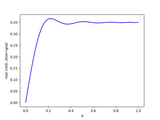
The sign function is also useful to approximate, e.g. for oblivious amplitude amplification. Running

pyqsp --plot-positive-only --plot --polyargs=19,10 --plot-real-only --polyname poly_sign poly

produces the QSP phase angles for a degree 19 polynomial approximation, using the error function of kappa * a, where kappa is 10, with a response function as shown in this plot:

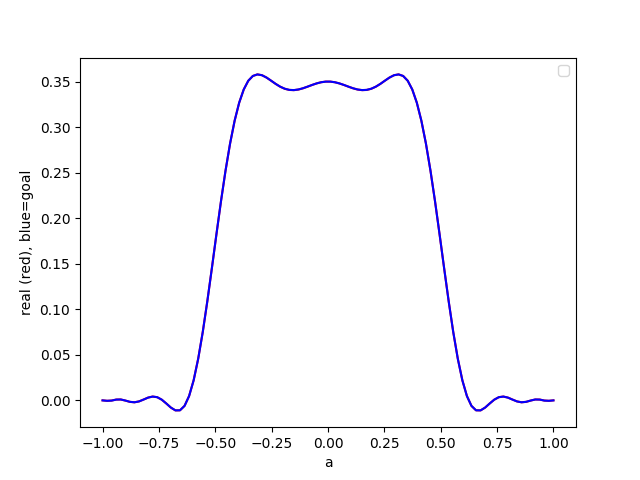
A threshold function is useful, for example, for distinguishing eigenvalues and singular values. Running

pyqsp --plot-real-only --plot --polyargs=20,20 --polyname poly_thresh poly

produces the QSP phase angles for a degree 20 polynomial approximation, using two error functions kappa 20, with a response function as shown in this plot:

Sine and cosine functions are useful, for example, for Hamiltonian simulation. Running:

pyqsp --plot --func "np.cos(3*x)" --polydeg 6 --plot-qsp-model polyfunc

produces the QSP phase angles for a degree 6 polynomial approximation of cos(3*x), and produces this plot:

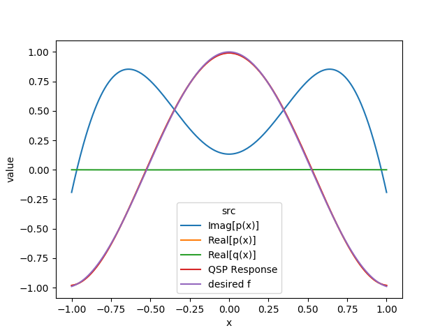
This example also shows how an arbitrary function can be specified (using a numpy expression) as a string, and fit using an arbitrary order polynomial (may need to be even or odd, to match the function), using optimization via tensorflow, and a keras model. The example also shows an alternative style of plot, produced using the --plot-qsp-model flag.

Code design

• angle_sequence.py is the main module of the algorithm.
• LPoly.py defines two classes LPoly and LAlg, representing Laurent polynomials and Low algebra elements respectively.
• completion.py describes the completion algorithm: Given a Laurent polynomial element $F(\tilde{w})$, find its counterpart $G(\tilde{w})$ such that $F(\tilde{w})+G(\tilde{w})*iX$ is a unitary element.
• decomposition.py describes the halving algorithm: Given a unitary parity Low algebra element $V(\tilde{w})$, decompose it as a unique product of degree-0 rotations $\exp{i\theta X}$ and degree-1 monomials $w$.
• ham_sim.py shows an example of how the angle sequence for Hamiltonian simulation can be found.
• response.py computes QSP response functions and generates plots
• poly.py provides some utility polynomials, namely the approximation of 1/a using a linear combination of Chebyshev polynomials
• main.py is the main entry point for command line usage
• qsp_model is the submodule providing generation of QSP phase angles using tensorflow + keras

The code is structured such that tensorflow is not imported by default, so that the package can be run without tensorflow being installed. If qsp_model is used, then tensorflow is required.

Requirements

This package can be run without tensorflow, if the qsp_model code is not used. If qsp_model is desired, then also install the requirements specified in tf_requirements.txt

Unit tests

A set of unit tests is also provided. Run them using python setup.py test

The qsp_model code depends on having tensorflow installed, and the unit tests for this code take awhile to run, so they are not run by default. To enable unit tests for this code, first do export PYQSP_TEST_QSP_MODELS=1

The qsp_model code unit tests can be run by themselves using python setup.py test -s pyqsp.test.test_qsp_models

Programmatic usage

To find the QSP angle sequence corresponding to a real Laurent polynomial $A(\tilde{w}) = \sum_{i=-n}^n a_i\tilde{w}^i$, simply run:

from pyqsp.angle_sequence import QuantumSignalProcessingPhases
ang_seq = QuantumSignalProcessingPhases([a_{-n}, a_{-n+2}, ..., a_n], signal_operator="Wz")
print(ang_seq)

To find the QSP angle sequence corresponding to a real (non-Laurent) polynomial $A(x) = \sum_{i=0}^n a_i x^i$, simply run:

from pyqsp.angle_sequence import QuantumSignalProcessingPhases
ang_seq = QuantumSignalProcessingPhases([a_{0}, a_{1}, ..., a_n], signal_operator="Wx")
print(ang_seq)

By default, QuantumSignalProcessingPhases uses the "laurent" method, which is typically quite fast, but can become unstable at very high orders of polynomials, due to numerical roundoff errors, and the need for some randomization in completing the polynomials.

QuantumSignalProcessingPhases can also be instructed to use the "tf" method, which employs tensorflow with a keras model, to find QSP phase angles using optimization. This stably finds very high-quality solutions, but can be quite slow, particularly compared with the "laurent" method. Do this, for example, using:

ang_seq = QuantumSignalProcessingPhases(poly, signal_operator="Wx", method="tf")

Note that with the "tf" method, only the "Wx" signal_operator model is supported. With this method, the polynomial can be a numpy Polynomial instance, or an instance of pyqsp.poly.StringPolynomial, e.g.

poly = StringPolynomial("np.cos(3*x)", 6)
ang_seq = QuantumSignalProcessingPhases(poly, method="tf")

You can also plot the response given by a given QSP angle sequence, e.g. using:

pyqsp.response.PlotQSPResponse(ang_seq, target=poly, signal_operator="Wx")

Command line usage

usage: pyqsp [-h] [-v] [-o OUTPUT] [--signal_operator SIGNAL_OPERATOR] [--plot] [--hide-plot] [--return-angles] [--poly POLY] [--func FUNC]
             [--polydeg POLYDEG] [--tau TAU] [--epsilon EPSILON] [--seqname SEQNAME] [--seqargs SEQARGS] [--polyname POLYNAME] [--polyargs POLYARGS]
             [--plot-magnitude] [--plot-probability] [--plot-real-only] [--title TITLE] [--measurement MEASUREMENT] [--output-json]
             [--plot-positive-only] [--plot-tight-y] [--plot-npts PLOT_NPTS] [--tolerance TOLERANCE] [--method METHOD] [--plot-qsp-model]
             [--phiset PHISET] [--nepochs NEPOCHS] [--npts-theta NPTS_THETA]
             cmd

usage: pyqsp [options] cmd

Version: 0.1.4
Commands:

    poly2angles - compute QSP phase angles for the specified polynomial (use --poly)
    hamsim      - compute QSP phase angles for Hamiltonian simulation using the Jacobi-Anger expansion of exp(-i tau sin(2 theta))
    invert      - compute QSP phase angles for matrix inversion, i.e. a polynomial approximation to 1/a, for given delta and epsilon parameter values
    angles      - generate QSP phase angles for the specified --seqname and --seqargs
    poly        - generate QSP phase angles for the specified --polyname and --polyargs, e.g. sign and threshold polynomials
    polyfunc    - generate QSP phase angles for the specified --func and --polydeg using tensorflow + keras optimization method (--tf)
    response    - generate QSP polynomial response functions for the QSP phase angles specified by --phiset

Examples:

    pyqsp --poly=-1,0,2 poly2angles
    pyqsp --poly=-1,0,2 --plot poly2angles
    pyqsp --signal_operator=Wz --poly=0,0,0,1 --plot  poly2angles
    pyqsp --plot --tau 10 hamsim
    pyqsp --plot --tolerance=0.01 --seqargs 3 invert
    pyqsp --plot-npts=4000 --plot-positive-only --plot-magnitude --plot --seqargs=1000,1.0e-20 --seqname fpsearch angles
    pyqsp --plot-npts=100 --plot-magnitude --plot --seqargs=23 --seqname erf_step angles
    pyqsp --plot-npts=100 --plot-positive-only --plot --seqargs=23 --seqname erf_step angles
    pyqsp --plot-real-only --plot --polyargs=20,20 --polyname poly_thresh poly
    pyqsp --plot-positive-only --plot --polyargs=19,10 --plot-real-only --polyname poly_sign poly
    pyqsp --plot-positive-only --plot-real-only --plot --polyargs 20,3.5 --polyname gibbs poly
    pyqsp --plot-positive-only --plot-real-only --plot --polyargs 20,0.2,0.9 --polyname efilter poly
    pyqsp --plot-positive-only --plot --polyargs=19,10 --plot-real-only --polyname poly_sign --method tf poly
    pyqsp --plot --func "np.cos(3*x)" --polydeg 6 polyfunc
    pyqsp --plot --func "np.cos(3*x)" --polydeg 6 --plot-qsp-model polyfunc
    pyqsp --plot-positive-only --plot-real-only --plot --polyargs 20,3.5 --polyname gibbs --plot-qsp-model poly
    pyqsp --polydeg 16 --measurement="z" --func="-1+np.sign(1/np.sqrt(2)-x)+ np.sign(1/np.sqrt(2)+x)" --plot polyfunc

positional arguments:
  cmd                   command

optional arguments:
  -h, --help            show this help message and exit
  -v, --verbose         increase output verbosity (add more -v to increase versbosity)
  -o OUTPUT, --output OUTPUT
                        output filename
  --signal_operator SIGNAL_OPERATOR
                        QSP sequence signal_operator, either Wx (signal is X rotations) or Wz (signal is Z rotations)
  --plot                generate QSP response plot
  --hide-plot           do not show plot (but it may be saved to a file if --output is specified)
  --return-angles       return QSP phase angles to caller
  --poly POLY           comma delimited list of floating-point coeficients for polynomial, as const, a, a^2, ...
  --func FUNC           for tf method, numpy expression specifying ideal function (of x) to be approximated by a polynomial, e.g. 'np.cos(3 * x)'
  --polydeg POLYDEG     for tf method, degree of polynomial to use in generating approximation of specified function (see --func)
  --tau TAU             time value for Hamiltonian simulation (hamsim command)
  --epsilon EPSILON     parameter for polynomial approximation to 1/a, giving bound on error
  --seqname SEQNAME     name of QSP phase angle sequence to generate using the 'angles' command, e.g. fpsearch
  --seqargs SEQARGS     arguments to the phase angles generated by seqname (e.g. length,delta,gamma for fpsearch)
  --polyname POLYNAME   name of polynomial generate using the 'poly' command, e.g. 'sign'
  --polyargs POLYARGS   arguments to the polynomial generated by poly (e.g. degree,kappa for 'sign')
  --plot-magnitude      when plotting only show magnitude, instead of separate imaginary and real components
  --plot-probability    when plotting only show squared magnitude, instead of separate imaginary and real components
  --plot-real-only      when plotting only real component, and not imaginary
  --title TITLE         plot title
  --measurement MEASUREMENT
                        measurement basis if using the polyfunc argument
  --output-json         output QSP phase angles in JSON format
  --plot-positive-only  when plotting only a-values (x-axis) from 0 to +1, instead of from -1 to +1 
  --plot-tight-y        when plotting scale y-axis tightly to real part of data
  --plot-npts PLOT_NPTS
                        number of points to use in plotting
  --tolerance TOLERANCE
                        error tolerance for phase angle optimizer
  --method METHOD       method to use for qsp phase angle generation, either 'laurent' (default) or 'tf' (for tensorflow + keras)
  --plot-qsp-model      show qsp_model version of response plot instead of the default plot
  --phiset PHISET       comma delimited list of QSP phase angles, to be used in the 'response' command
  --nepochs NEPOCHS     number of epochs to use in tensorflow optimization
  --npts-theta NPTS_THETA
                        number of discretized values of theta to use in tensorflow optimization

Example: plot response polynomial functions for sin(a) approximation

pyqsp --plot-qsp-model --phiset="[-1.63276817 0.20550406 -0.84198335  0.39732059 -0.26820613 2.41324245  0.04662674 -2.02847501 1.11311765  0.04662674 -0.72835021 -0.26820613 0.39732059 -0.84198335  0.20550406 -0.06197184]" response

History

• v0.0.3: initial version, with phase angle generation entirely done using https://arxiv.org/abs/2003.02831
• v0.1.0: added generation of phase angles using optimization via tensorflow (qsp_model code by Jordan Docter and Zane Rossi)
• v0.1.1: add tf unit tests to test_main; readme updates
• v0.1.2: fixed bug in qsp_model plotting (Re[q] wasn't being correctly computed for the qsp_model plot); made tf an optional requirement
• v0.1.3: fixed bug in qsp_model.qsp_layers - Re[q] is actually proportional to Imag[u[0,1]]; allow --nepochs and --npts-theta to be specified
• v0.1.4: add measurement basis option for qsp_models; add phase estimation polynomial