Linear time-variant model predictive control in Python.

Project description
qpmpc


Model predictive control (MPC) in Python for optimal-control problems that are quadratic programs (QP). This includes linear time-invariant (LTI) and time-variant (LTV) systems with linear constraints. The corresponding QP has the form:

This module is designed for prototyping. If you need performance, check out the alternatives below.
Installation
pip install qpmpc
Usage
This module defines a one-stop shop function:
solve_mpc(problem: MPCProblem, solver: str) -> Plan
The MPCProblem defines the model predictive control problem (LTV system, LTV constraints, initial state and cost function to optimize) while the returned Plan holds the state and input trajectories that result from optimizing the problem (if a solution exists). The solver string is used to select the backend quadratic programming solver.
Example
Let us define a triple integrator:
    import numpy as np

    horizon_duration = 1.0  # [s]
    N = 16  # number of discretization steps
    T = horizon_duration / N
    A = np.array([[1.0, T, T ** 2 / 2.0], [0.0, 1.0, T], [0.0, 0.0, 1.0]])
    B = np.array([T ** 3 / 6.0, T ** 2 / 2.0, T]).reshape((3, 1))
Suppose for the sake of example that acceleration is the main constraint acting on our system. We thus define an acceleration constraint |acceleration| <= max_accel:
    max_accel = 3.0  # [m] / [s] / [s]
    accel_from_state = np.array([0.0, 0.0, 1.0])
    C = np.vstack([+accel_from_state, -accel_from_state])
    e = np.array([+max_accel, +max_accel])
This leads us to the following linear MPC problem:
    from qpmpc import MPCProblem

    x_init = np.array([0.0, 0.0, 0.0])
    x_goal = np.array([1.0, 0.0, 0.0])
    problem = MPCProblem(
        transition_state_matrix=A,
        transition_input_matrix=B,
        ineq_state_matrix=C,
        ineq_input_matrix=None,
        ineq_vector=e,
        initial_state=x_init,
        goal_state=x_goal,
        nb_timesteps=N,
        terminal_cost_weight=1.0,
        stage_state_cost_weight=None,
        stage_input_cost_weight=1e-6,
    )
We can solve it with:
    from qpmpc import solve_mpc

    solution = solve_mpc(problem, solver="proxqp")
The solution holds complete state and input trajectories as stacked vectors. For instance, we can plot positions, velocities and accelerations as follows:
    import pylab

    t = np.linspace(0.0, horizon_duration, N + 1)
    X = solution.states
    positions, velocities, accelerations = X[:, 0], X[:, 1], X[:, 2]
    pylab.ion()
    pylab.plot(t, positions)
    pylab.plot(t, velocities)
    pylab.plot(t, accelerations)
    pylab.grid(True)
    pylab.legend(("position", "velocity", "acceleration"))
This example produces the following trajectory:
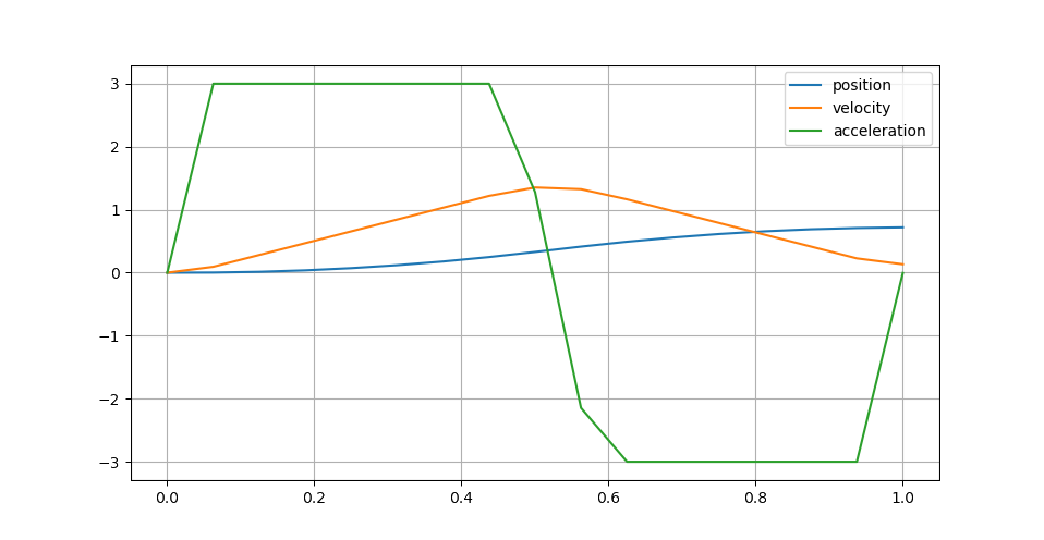
The behavior is a weighted compromise between reaching the goal state (weight 1.0) and keeping reasonable finite jerk inputs (weight 1e-6). The latter mitigate bang-bang accelerations but prevent fully reaching the goal within the horizon. See the examples folder for more examples.
Areas of improvement
This module is incomplete with regards to the following points:
- Cost functions: can be extended to general linear stage cost functions
- Documentation: there are some undocumented functions
- Test coverage: only one end-to-end test
Check out the contribution guidelines if you are interested in lending a hand.
Alternatives
This module is designed for faster prototyping rather than performance. You can also check out the following open-source libraries:
| Name | Systems | Languages | License |
|---|---|---|---|
| Copra (LTV fork) | Linear time-variant | Python/C++ | BSD-2-Clause |
| Copra (original) | Linear time-invariant | Python/C++ | BSD-2-Clause |
| Crocoddyl | Nonlinear | Python/C++ | BSD-3-Clause |
| mpc-interface | Linear time-variant | Python/C++ | BSD-2-Clause |
| pyMPC | Linear time-variant | Python | MIT |
Release history Release notifications | RSS feed


Download files
Download the file for your platform. If you're not sure which to choose, learn more about installing packages.


