Embed gnuplot, ditaa, pyplot, DOT, etc. diagrams in your Sphinx-based documentation.

Project description
A sphinx extension to plot all kind of graph such as ditaa/gnuplot/pyplot, etc. within .rst file.
Usage: Inline diagram, show as svg:
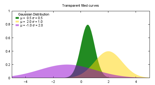
.. plot:: gnuplot
    :caption: figure 3. illustration for gnuplot
    :size: 500,300

    set style fill transparent solid 0.5 noborder
    set style function filledcurves y1=0

    Gauss(x,mu,sigma) = 1./(sigma*sqrt(2*pi)) * exp( -(x-mu)**2 / (2*sigma**2) )
    d1(x) = Gauss(x, 0.5, 0.5)
    d2(x) = Gauss(x,  2.,  1.)
    d3(x) = Gauss(x, -1.,  2.)

    set xrange [-5:5]
    set yrange [0:1]
    set key title "Gaussian Distribution"
    set key top left Left reverse samplen 1
    set title "Transparent filled curves"
    plot d1(x) fs solid 1.0 lc rgb "forest-green" title "μ =  0.5 σ = 0.5", \
         d2(x) lc rgb "gold" title "μ =  2.0 σ = 1.0", \
         d3(x) lc rgb "dark-violet" title "μ = -1.0 σ = 2.0"
1. Installing and setup
pip install sphinxcontrib-plot
And just add sphinxcontrib.plot to the list of extensions in the conf.py file. For example:
extensions = ['sphinxcontrib.plot']
2. Introduction and examples
In rst we we use image and figure directive to render image/figure. In fact we can plot anything in rst as it was on shell. For examples:
2.1 gnuplot example
The first example is gnuplot.:
.. plot:: gnuplot
    :caption: figure 3. illustration for gnuplot
    :size: 500,300

    set style fill transparent solid 0.5 noborder
    set style function filledcurves y1=0

    Gauss(x,mu,sigma) = 1./(sigma*sqrt(2*pi)) * exp( -(x-mu)**2 / (2*sigma**2) )
    d1(x) = Gauss(x, 0.5, 0.5)
    d2(x) = Gauss(x,  2.,  1.)
    d3(x) = Gauss(x, -1.,  2.)

    set xrange [-5:5]
    set yrange [0:1]
    set key title "Gaussian Distribution"
    set key top left Left reverse samplen 1
    set title "Transparent filled curves"
    plot d1(x) fs solid 1.0 lc rgb "forest-green" title "μ =  0.5 σ = 0.5", \
         d2(x) lc rgb "gold" title "μ =  2.0 σ = 1.0", \
         d3(x) lc rgb "dark-violet" title "μ = -1.0 σ = 2.0"
After convert using gnuplot, the above file becomes:
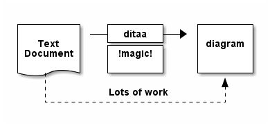
2.1 ditaa example
Another example is ditaa. ditaa is a small command-line utility that can convert diagrams drawn using ascii art into proper bitmap graphics. Ditaa is in java and we We could use following directive to render the image with extra parameters:
.. plot:: ditaa
   :caption: figure 1. illustration for ditaa

    +--------+   +-------+    +-------+
    |        | --+ ditaa +--> |       |
    |  Text  |   +-------+    |diagram|
    |Document|   |!magic!|    |       |
    |     {d}|   |       |    |       |
    +---+----+   +-------+    +-------+
        :                         ^
        |       Lots of work      |
        +-------------------------+
Or plot it with parameters:
.. plot:: ditaa --svg
   :caption: figure 2. illustration for ditaa with option

      +--------+   +-------+    +-------+
      |        | --+ ditaa +--> |       |
      |  Text  |   +-------+    |diagram|
      |Document|   |!magic!|    |       |
      |     {d}|   |       |    |       |
      +---+----+   +-------+    +-------+
          :                         ^
          |       Lots of work      |
          +-------------------------+
After convert using ditaa, the above file becomes:
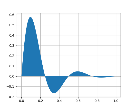
2.3 python example
Another example is mulplotlib.plot.
.. plot:: python
    :caption: figure 4. illustration for python

    import numpy as np
    import matplotlib.pyplot as plt

    x = np.linspace(0, 1, 500)
    y = np.sin(4 * np.pi * x) * np.exp(-5 * x)

    fig, ax = plt.subplots()

    ax.fill(x, y, zorder=10)
    ax.grid(True, zorder=5)
    plt.show()
After conversion using python, we could get the following image:
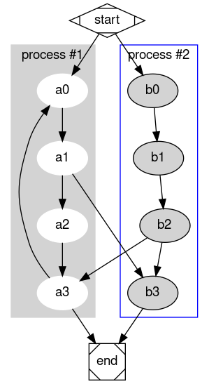
2.4 graphviz(dot) example
Another example is graphivx(dot), since we want to generate png image, we add the option in the command, it’s dot’s own option:
.. plot:: dot -Tpng
    :caption: illustration for dot

    digraph G {

            subgraph cluster_0 {
                    style=filled;
                    color=lightgrey;
                    node [style=filled,color=white];
                    a0 -> a1 -> a2 -> a3;
                    label = "process #1";
            }

            subgraph cluster_1 {
                    node [style=filled];
                    b0 -> b1 -> b2 -> b3;
                    label = "process #2";
                    color=blue
            }
            start -> a0;
            start -> b0;
            a1 -> b3;
            b2 -> a3;
            a3 -> a0;
            a3 -> end;
            b3 -> end;

            start [shape=Mdiamond];
            end [shape=Msquare];
    }
After convert using dot, the above file becomes:
2.5 convert example
Another example is convert. You can write the command in the commnad line:
.. plot::
:caption: illustration for convert

convert rose:  -fill none -stroke white -draw 'line 5,40 65,5'  rose_raw.png
This is the output:

or you can write most of the command line in the body:
.. plot::
:caption: illustration for convert
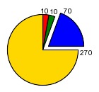
convert -size 140x130 xc:white -stroke black \
-fill red -draw "path 'M 60,70 L 60,20 A 50,50 0 0,1 68.7,20.8 Z'" \
-fill green -draw "path 'M 60,70 L 68.7,20.8 A 50,50 0 0,1 77.1,23.0 Z'" \
-fill blue -draw "path 'M 68,65 L 85.1,18.0 A 50,50 0 0,1 118,65 Z'" \
-fill gold -draw "path 'M 60,70 L 110,70 A 50,50 0 1,1 60,20 Z'" \
-fill black -stroke none -pointsize 10 \
-draw "text 57,19 '10' text 70,20 '10' text 90,19 '70' text 113,78 '270'" \
piechart.jpg
2.6 Other applications
In theory, All the command which could generate graph could be used after the directive “..plot::”. Please report it when you found anyone which works or doesn’t work.
3 Options
sphinxcontrib-plot provide some options for easy use.
3.1 command options
First of all, you can add any parameter after the command. sphinxcontrib-plot doesn’t know and interfere with it and only get the graph after it’s executed. for example:
.. plot:: ditaa --no-antialias -s 2
   :caption: figure 1. illustration for ditaa with option.

    +--------+   +-------+    +-------+
    |        | --+ ditaa +--> |       |
    |  Text  |   +-------+    |diagram|
    |Document|   |!magic!|    |       |
    |     {d}|   |       |    |       |
    +---+----+   +-------+    +-------+
        :                         ^
        |       Lots of work      |
        +-------------------------+
3.2 sphinxcontrib-plot options
sphinxcontrib-plot specific options:
- size:
Control the output image size for gnuplot.
- plot_format:
the output image format, for example svg, png, etc, overwrite global plot_format.
- convert:
use convert to add some watermark
- show_source:
for text generated iamge, if the source code is shown.
- caption:
The title for the image.
- hidden:
Only generate the image bug doesn’t render it in the document.
Common image options:
Since plot generate figure/image, it’s in fact a image. So all the options of figure and image could be used. For example:
- name:
the reference name for the figure/image. For html, it would rename the output file to the @name. Since latex doesn’t do well in supporting :name: for example doesn’t support Chinese/SPACE, doesn’t generate linke to :name, we don’t do that in latex.
For example:
.. plot:: gnuplot
    :caption: figure 1. illustration for gnuplot with watermark.
    :name: figure 1. illustration for gnuplot with watermark.
    :convert: -stroke red -strokewidth 2 -fill none -draw "line 100,100
             200, 200"
    :size: 900,600
    :width: 600

    plot [-5:5] (sin(1/x) - cos(x))*erfc(x)
3.2 global options
Please add the following option into you conf.py to designate defualt output file format for different targe. The default output format for html and latex is as following, you can change them in you own conf.py:
plot_format = dict(html='svg', latex='pdf')
If it doesn’t support suck kind of output format, it would fall back to .png.
4. License
GPLv3
5. Changelog
1.0 Initial upload. 1.0.8 Bug fix: When there is no :size: in gnuplot plot, it might crash. 1.0.10 Bug fix: fix the issue that convert doesn’t work. 1.0.12 Support magick script
Release history Release notifications | RSS feed


Download files
Download the file for your platform. If you're not sure which to choose, learn more about installing packages.
Source Distribution
Hashes for sphinxcontrib-plot-1.0.12.tar.gz
| Algorithm | Hash digest | |
|---|---|---|
| SHA256 | d299fffe403bb01055458f60f4693ef09facd4273010353c409e1f5a1bc70f71 |
|
| MD5 | af97922feb7a509d4cdfae4d352aa317 |
|
| BLAKE2b-256 | 91c37ff277f01defb7818cbc003e4ab99f744512c614b7329e8e05117f504899 |


