Spike sorting based on Gaussian Mixture Model

Project description
DESCRIPTION
Spiky allows you to sort spikes from single electrodes. The clustering is performed with Gaussian Mixture Model (GMM) and vanilla Expectation-Maximization (EM) algorithm. To penalize complexity we use Bayesian Information Criterion (BIC).
Spiky allows you to run a confusion test to evaluate how prone to misclassification the clusters are. And also provides a cuantitative meassure of how far each cluster is from the rest. This two tools allow us to get a better intuition about the validity of the results.
Please check our “Turorial section” to get an intuition of what Spiky is capable of. And don’t forget to keep an eye on the “Description Section” in order to understand how Spiky works.
INSTALATION
Spiky is available through pypi so if you are runing python in your computer, go ahead and type in the terminal:
pip install Spiky
If you need python, we strongly recommend you to install “conda” first. (What is conda?: conda is a package and enviroment manager. It will keep things tight and clean).
“Conda” instalation:
For Windows users:
go to: https://conda.io/miniconda.html and download miniconda (for python=3, windows)
Double-click the .exe file.
Follow the instructions on the screen.
When installation is finished, from the Start menu, open the Anaconda Prompt.
For Linux users:
go to: https://conda.io/miniconda.html and download miniconda (for python=3, Linux)
Open terminal and use the “cd” command to navegate to the folder where you downloaded your miniconda file
type: “bash Miniconda3-latest-Linux-x86_64.sh”
Follow the prompts on the installer screens.
To make the changes take effect, close and then re-open your Terminal window.
For Mac Users:
go to: https://conda.io/miniconda.html and download miniconda (for python=3, Mac)
Open terminal and use the “cd” command to navegate to the folder where you downloaded your miniconda file
type: “bash Miniconda3-latest-MacOSX-x86_64.sh”
Follow the prompts on the installer screens.
To make the changes take effect, close and then re-open your Terminal window.
NOTE: matplotlib needs a framework build to work properly with conda. A workaround this problem is type in terminal:
conda install python.app
Use “pythonw” rather than “python” to run python code
Now that you have conda already installed, open a terminal and type:
conda create –name snowflake python=3
source activate snowflake
pip install Spiky
(Note: we encourage you to pick a different name for your virtual environment. We used “snowflake” just as an example)
Now you can test Spiky by runing one of the available examples. Go to TUTORIAL for instructions
TUTORIAL
Copy the folder called “buzsaki” that is under “examples” and paste it in your computer’s desktop. The folder contains a dataset obtained from BuzsakiLabs. By the way, have you checked his webpage? If you haven’t done it yet, here is the link http://buzsakilab.com/wp/
The dataset we have choosen is the simultaneous intracellular and extracellular recording from the hippocampus of anesthetized rats hc-1 ‘d533101.dat’ which is a good starting point (you can play with other examples later). You can find the dataset details here:
Henze, DA; Harris, KD; Borhegyi, Z; Csicsvari, J; Mamiya, A; Hirase, H; Sirota, A; Buzsáki, G (2009): Simultaneous intracellular and extracellular recordings from hippocampus region CA1 of anesthetized rats. CRCNS.org.http://dx.doi.org/10.6080/K02Z13FP
Now, open a terminal, navegate up to “buzsaki” folder and type:
python buzsaki.py
The terminal will prompt you with some general information like these:
Preprocesing
Simultaneous spikes deleted: 144
Interpolated spike deleted: 11
Threshold: 130.47
Detected peaks: 2977
Extra features: Energy, Amplitud, Area
Preprocessing time: 2.45 sec.
DONE
Clustering
100% | Elapsed Time: 0:00:04|################|Time: 0:00:04 | Neurons: 4
Clusters found: 4
Clustering time: 6.80 sec.
L-ratios:
0: 0.01
1: 0.00
2: 10.30
3: 0.01
DONE
When the process is finished, you should see a picture like the one below showing the different spikes grouped by cluster:
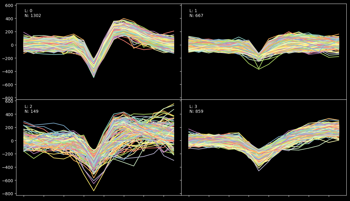
The algorithm has found 4 clusters. We know from ground truth (provided by BuzsakiLabs in the form of intracellular recording) that the efficiency of the result is arround 90% (because we have found 860 spikes under the fourth label but the intercellular record shows that there were actually 960 spikes). What happened with the rest? Well some of the spikes just don’t show up in the extracellular recording and a small fraction have been misclassified due to their low amplitud.
Lets now imagine for one second that we have no information about the grown truth. So, the first thing we should keep an eye on are the L-ratios displayed above. We can see that all of them except the third one are very low (which is good, it means that the clusters are far away from each other in terms of mahalanobis distance). So, to understand what is really going on, we will have to run a blur test.
Please, close the previews plot and wait for the blur test to finish. A print like this will be shown:
- Bluring
100% | Elapsed Time: 0:00:04|################|Time: 0:00:04 | Neurons: 4 DONE
And finally, a confusion matrix will appear on screen:
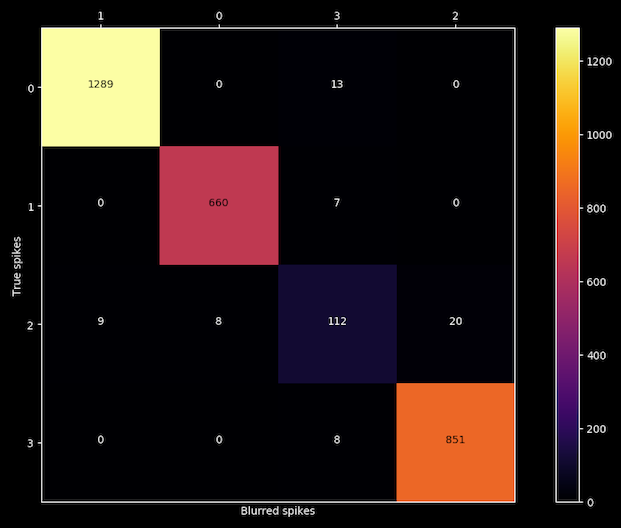
Now we can confirm our first intuition about the accuracy of the third cluster because after blurring each spikes with the noise of its own cluster, the algorithm is able to reproduce the same results for clusters 0, 1 and 3 but is confusing labels on cluster number 2, so we got our liar.
Documentation
REFERENCES
Preprosesing of data is handled as described by:
Quian Quiroga R, Nadasdy Z, Ben-Shaul Y (2004) Unsupervised Spike Detection and Sorting with Wavelets and Superparamagnetic Clustering. Neural Comp 16:1661-1687.
L-ratio calculation is computed following:
Schmitzer-Torbert et al. Quantitative measures of cluster quality for use in extracellular recordings Neuroscience 131 (2005) 1–11 11
Confusion Matrix calculation is computed acording to:
Alex H. Barnetta, Jeremy F. Maglandb, Leslie F. Greengardc Validation of neural spike sorting algorithms without ground-truth information Journal of Neuroscience Methods 264 (2016) 65–77
Example dataset was obtained from:
Henze, DA; Harris, KD; Borhegyi, Z; Csicsvari, J; Mamiya, A; Hirase, H; Sirota, A; Buzsáki, G (2009): Simultaneous intracellular and extracellular recordings from hippocampus region CA1 of anesthetized rats. CRCNS.org.http://dx.doi.org/10.6080/K02Z13FP


Download files
Download the file for your platform. If you're not sure which to choose, learn more about installing packages.
Source Distribution
Built Distribution
Hashes for spiky-1.0.2-py2.py3-none-any.whl
| Algorithm | Hash digest | |
|---|---|---|
| SHA256 | caeb08984619398f2b871399a852bea8aec351d4f364968c0352864a2303ef5c |
|
| MD5 | f371f8259a31209d4086754344be6490 |
|
| BLAKE2b-256 | 55992710c6f3575a83521d6d24161790a32a51db95077875ea82668362bc8344 |


