Spike sorting based on Gaussian Mixture Model

Project description
### **Spiky** - A Spike Sorting Package
---
### DESCRIPTION
---
**Spiky** will allow you to sort spikes from single electrodes. The clustering is performed by a Gaussian Mixture Model (GMM) and vanilla Expectation-Maximization (EM) algorithm. To penalize complexity we are using Bayesian Information Criterion (BIC).
**Spiky** is able to run confusion tests to evaluate how prone to misclassification the clusters are. And also provides a cuantitative meassure of how far each cluster is from the rest (in terms of mahalanobis distance).
Please check our "Turorial section" to get an intuition of how to run **Spiky**. And don't forget to keep an eye on the "Description Section" to understand how **Spiky** works.
---
### INSTALATION
---
**Spiky** is available through pypi so if you are runing python in your computer, go ahead and type in terminal:
- pip install Spiky
If you need python, we strongly recommend you to install **"conda"**. (What is conda?: conda is a package and enviroment manager. It will keep things tight and clean).
"Conda" installation:
On WINDOWS:
- go to: https://conda.io/miniconda.html and download miniconda.
- Double-click the .exe file.
- Follow the instructions on the screen.
- When installation is finished, from the Start menu,
open the Anaconda Prompt.
On LINUX:
- go to: https://conda.io/miniconda.html and download miniconda.
- Open terminal and use the "cd" command to navegate to the folder
where you downloaded your miniconda file
- type: "bash Miniconda3-latest-Linux-x86_64.sh"
- Follow the prompts on the installer screens.
- To make the changes take effect, close and then re-open your
Terminal window.
On MAC:
- go to: https://conda.io/miniconda.html and download miniconda
- Open terminal and use the "cd" command to navegate to the folder
where you downloaded your miniconda file
- type: "bash Miniconda3-latest-MacOSX-x86_64.sh"
- Follow the prompts on the installer screens.
- To make the changes take effect, close and then re-open your
Terminal window.
NOTE: matplotlib needs a framework build to work properly with conda.
A workaround for this problem is obtained by type in terminal:
- conda install python.app
- Use "pythonw" rather than "python" to run python code
Spiky installation:
Open a terminal and type what comes next:
- conda create --name snowflake python=3
- source activate snowflake
- pip install Spiky
Note: we encourage you to pick a different name for your virtual
environment. We used "snowflake" just as an example
Now you can test **Spiky** by runing one of the available examples. Go to TUTORIAL for instructions
---
### TUTORIAL
---
#### Buzsaki dataset
Copy the folder called "buzsaki" that is under "examples" and paste it in your computer's desktop. The folder contains a dataset obtained from BuzsakiLabs. By the way, have you checked his webpage? If you haven't done it yet, here is the [link]( http://buzsakilab.com/wp/)
The dataset we have choosen is the simultaneous intracellular and extracellular recording from the hippocampus of anesthetized rats hc-1 'd533101.dat' which is a good starting point (you can play with other examples later). You can find the dataset details here:
- Henze, DA; Harris, KD; Borhegyi, Z; Csicsvari, J; Mamiya, A; Hirase, H; Sirota, A; Buzsáki, G (2009): Simultaneous intracellular and extracellular recordings from hippocampus region CA1 of anesthetized rats. CRCNS.org. [link](http://dx.doi.org/10.6080/K02Z13FP)
Now, open a terminal, navegate up to "buzsaki" folder and type:
python buzsaki.py
The terminal will prompt you with some general information like these:
Preprocesing
Simultaneous spikes deleted: 144
Interpolated spike deleted: 11
Threshold: 130.47
Detected peaks: 2977
Extra features: Energy, Amplitud, Area
Preprocessing time: 2.45 sec.
DONE
Clustering
100% | Elapsed Time: 0:00:04|################|Time: 0:00:04 | Neurons: 4
Clusters found: 4
Clustering time: 3.80 sec.
L-ratios:
0: 0.01
1: 0.00
2: 10.30
3: 0.01
DONE
When the process is finished, you should see a picture like the one below showing the different spikes grouped by cluster:
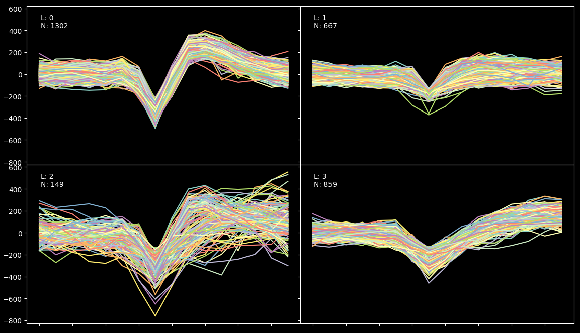
The algorithm has found 4 clusters. We know from ground truth (provided by BuzsakiLabs in the form of intracellular recording) that the efficiency of the result is arround 90% (because we have found 860 spikes under the fourth label but the intercellular record shows that there were actually 960 spikes). What happened with the rest? Well some of the spikes just don't show up in the extracellular recording and a small fraction have been misclassified due to their low amplitud.
Lets now imagine for one second that we have no information about the grown truth. So, the first thing we should keep an eye on are the L-ratios displayed above. We can see that all of them except the third one are very low (which is good, it means that the clusters are far away from each other in terms of mahalanobis distance). So, to understand what is really going on, we will have to run a blur test.
Please, close the previews plot and wait for the blur test to finish. A print like this will be shown:
Bluring
100% | Elapsed Time: 0:00:04|################|Time: 0:00:04 | Neurons: 4
DONE
And finally, a confusion matrix will appear on screen:
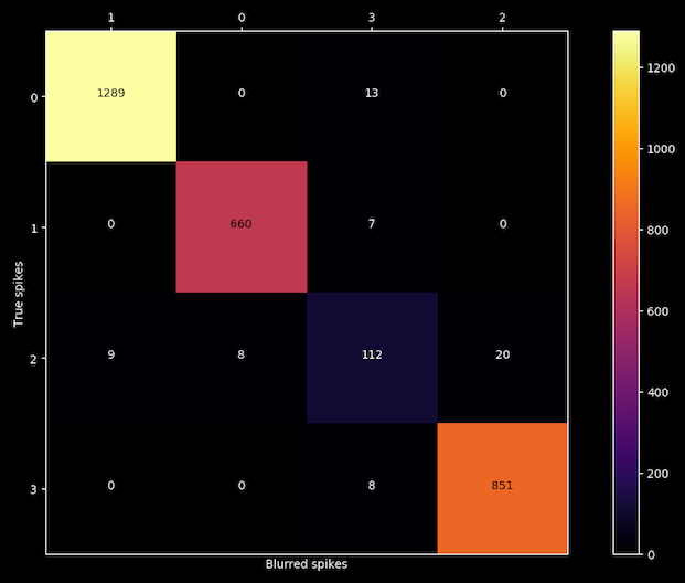
After blurring each spike with the noise of its own cluster, the algorithm is able to reproduce the results for clusters 0, 1 and 3 but is confusing labels on cluster number 2, so we got our liar.
#### Quiroga dataset
Copy the folder called "Quiroga" that is inside "examples" and paste it in your computer's desktop. The folder contains a dataset obtained from the Centre for Systems Neuroscience at the University of Leicester. Take a moment to check their [webpage](https://www2.le.ac.uk/centres/csn)
The dataset we have choosen is from simulated recording and are available [here](https://www2.le.ac.uk/centres/csn/research-2/spike-sorting):
Now, open a terminal, navegate up to "Quiroga" folder and type:
`python quiroga.py`
The terminal will prompt you with some general information like these:
parameters/parameters.json file loaded correctly.
Preprocesing
Simultaneous spikes deleted: 85
Interpolated spike deleted: 4
Threshold: 106.75
Detected peaks: 3336
Extra features: Energy, Amplitud, Area
Preprocessing time: 2.91 sec.
DONE
Clustering
100% | Elapsed Time: 0:00:03|################|Time: 0:00:03 | Neurons: 5
Clusters found: 5
CLustering time: 6.61 sec.
L-ratios:
0: 29.42
1: 0.00
2: 0.00
3: 0.00
4: 17.12
DONE
When the process is finished, you should see a picture like the one below showing the different spikes grouped by cluster:
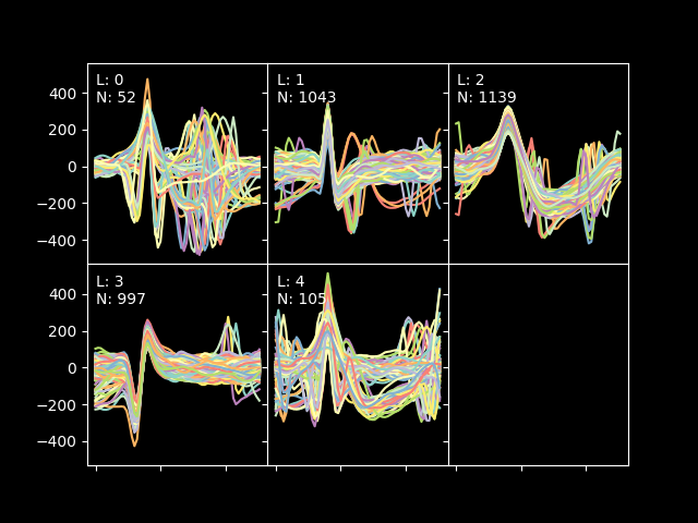
The algorithm has found 5 clusters, but ones again, the l-ratios are telling us that 2 of the clusters have spikes that are very close to them, so let's run a blurring test. Please, close the previews plot and wait for the blur test to finish. A print like this will be shown:
Bluring
100% | Elapsed Time: 0:00:02|################|Time: 0:00:02 | Neurons: 6
DONE
And finally, a confusion matrix will appear on screen:

We can see that two of the clusters are mixing spikes.
---
### DOCUMENTATION
---
#### spiky.New(pfile=‘None’, rfile=‘None’):
This is the class constructor. It will create
an instance of the main spiky class.
PARAMETERS
pfile : str
Path to the ‘.json’ file containing the parameters setting.
The name is a contraction for parameters_file
rfile : str
Path to the ‘.dat’ or ‘.mat’ file containing the raw data.
The name is a contraction for raw_data_file.
Notes :
Use integer 16 to represent the data (float is just a waste of resources).
The file must contain the data of one dataset, so if you have multiple electrodes
within the same file, split them up into different files.
ATTRIBUTES
Note: This attributes will be available ones you call "run" within the spiky object that you created.
prms : dict
Dictionary containing the parameters setting.
raw : ndarray
Dataset array
thres : float
Threshold level for spike detection
pks : ndarray
Array containing the time of spikes
spks : ndarray
Spikes time series
wvSpks : ndarray
Wavelet decomposition of spikes
extFeat : ndarray
Array containing extra features such as Amplitud, Energy, Area
X : ndarray
Array containing normalized features for clustering
gmm : Gaussian mixture class object
The gaussian mixture object
labels : ndarray
Array containing the labels for each spike
lr : ndarray
L-ratios for each cluster
#### spiky.New.loadParams(pfile=‘None’):
Loads the ‘.json’ file containing the parameters setting.
pfile : str
Path to parameters '.json' file
#### spiky.New.loadRawArray(rarray):
Loads an array containing the data set.
rarray : ndarray
Array containing the dataset
#### spiky.New.loadRawFile(rfile):
Loads a ‘.mat’ or ‘.dat’ file containing the data set.
rfile : str
Path to the ‘.dat’ or ‘.mat’ file containing the raw data.
#### spiky.New.filter():
Filters dataset using cascaded second-order sections digital
IIR filter defined by sos. The parameters are taken from the
‘.json’ configuration file. The filter is zero phase-shift
#### spiky.New.run():
Main clustering method. The parameters are set as specified by ‘.json’ file.
#### spiky.New,plotClusters():
Plots spike clusters as found by “run” method.
#### spiky.New.blur():
Re-run the clustering algorithm after performing a
blur of spikes within same labels, and plots the
confusion matrix.
-------------
#### PARAMETERS FILE:
Traces:
- prms[“trace”][“name”] : Defines a name for this set of parameters
Spike detection:
- prms[“spkD”][“thres”] : Defines the threshold level (default = 4.
max/min=3.9-4.1 as defined by Quian-Quiroga paper)
- prms[“spkD”][“way”] : Defines if the algorithm will search for maximum or
minimums in the dataset. (values: “valley” - “peaks”)
- prms[“spkD”][“minD”] : Defines how many spaces between two consecutive peaks
there should be in order to take them as separated peaks.
- prms[“spkD”][“before”]: Defines how many spaces after the peak
will be taken to build the spike.
- prms[“spkD”][“after”] : Defines how many spaces before the peak will
be taken to build the spike.
Filtering:
- prms[“filt”][“q”] : Filters order.
- prms[“filt”][“hz”] : Nysquit frecuency.
- prms[“filt”][“low”] : Defines low frequency cut.
- prms[“filt”][“high”] : Defines High frequency cut.
Spike alignment:
- prms[“spkA”][“resol”] : Defines the resolution used to compute interpolation and
alignment (equal to the number of intermediate point taken
between two consecutive points in the spike
Spike errase:
- prms[“spkE”][“minD”] : Delete spike if it contains 2 peaks separated less than
“minD” positions and the relative amplitud of each one
is bigger than “lvl”.
- prms[“spkE”][“lvl”] : Delete spike if it contains 2 peaks separated less than
“minD” positions and the relative amplitud of each one
is bigger than “lvl”.
Wavelet decomposition:
- prms[“wv”][“lvl”] : Level of decomposition for multilevel wavelet decomposition.
- prms[“wv”][“func”] : Function to be used for wavelet decomposition.
- prms[“wv”][“mode”] : Boundary condition to use in wavelet decomposition
Clustering:
- prms[“gmm”][“maxK”] : Maximum number of clusters to look for solutions.
- prms[“gmm”][“ftrs”] : Number of features to take into account.
- prms[“gmm”][“maxCorr”]: Maximum correlation allowed between features
- prms[“gmm”][“inits”] : Number of random weights initializations
Blurring:
- prms[“blur”][“alpha”] : Blurring intensity (0-1)
---
### ACKNOWLEDGMENT
---
I would like to thank Eugenio Urdapilleta[<sup>1</sup>](https://www.researchgate.net/profile/Eugenio_Urdapilleta) and Damian Dellavale[<sup>2</sup>](https://www.researchgate.net/profile/Damian_Dellavale2) for their guidance.
---
### REFERENCES
---
Preprosesing of data is handled as described by:
- Quian Quiroga R, Nadasdy Z, Ben-Shaul Y (2004) **Unsupervised Spike Detection and Sorting with
Wavelets and Superparamagnetic Clustering**. Neural Comp 16:1661-1687.
L-ratio calculation is computed following:
- Schmitzer-Torbert et al. **Quantitative measures of cluster quality for use in extracellular recordings**
Neuroscience 131 (2005) 1–11 11
Confusion Matrix calculation is computed acording to:
- Alex H. Barnetta, Jeremy F. Maglandb, Leslie F. Greengardc **Validation of neural spike sorting
algorithms without ground-truth information** Journal of Neuroscience Methods 264 (2016) 65–77
Example dataset was obtained from:
- Henze, DA; Harris, KD; Borhegyi, Z; Csicsvari, J; Mamiya, A; Hirase, H; Sirota, A; Buzsáki, G (2009):
**Simultaneous intracellular and extracellular recordings from hippocampus region CA1 of anesthetized rats**.
CRCNS.org.http://dx.doi.org/10.6080/K02Z13FP


Download files
Download the file for your platform. If you're not sure which to choose, learn more about installing packages.
Source Distribution
spiky-1.0.3.tar.gz
(20.8 kB
view hashes)
Built Distribution
spiky-1.0.3-py2.py3-none-any.whl
(21.2 kB
view hashes)
Close
Hashes for spiky-1.0.3-py2.py3-none-any.whl
| Algorithm | Hash digest | |
|---|---|---|
| SHA256 | bdc905623e9e0e4a4efee5e7483b5800b9c67ffb0c9abc0e41681ce6eddad639 |
|
| MD5 | fff4dc5fa187484e2b034efda6a2913e |
|
| BLAKE2b-256 | 783cbb9dad297eaf964be381b5b72fa015aca3cdc2b7560f96a30297ce9b3b1a |


